RNA-seq Data Analysis
Jialin Ma
October 22, 2018
- Load the packages
- Load the dataset
- Regularized-logarithm transformation (rlog)
- Heatmap showing sample distance (rlog transformed)
- PCA plot (rlog transformed)
- Differential expression analysis
- MA plot
- Distribution of p values
- Annotating the gene names
- Generate a table of differentially expressed genes
- Gene clustering
- PCA plot of genes
- Pathway analysis
Load the packages
suppressPackageStartupMessages({
    library(here)
    library(dplyr)
    library(ggplot2)
    library(pheatmap)
    library(RColorBrewer)
    library(EnsDb.Hsapiens.v86)
    library(DESeq2)
})
Load the dataset
The transcript quantification results have been produced by salmon. The tximport package can import and summarize the information on gene level.
library(tximport)
tx2gene <- transcripts(EnsDb.Hsapiens.v86,
        return.type = "data.frame", columns = c("tx_id", "gene_id"))
salmon_dirs <- list.files(here("result/salmon_quant"), full.names = TRUE)
salmon_files <- sapply(salmon_dirs, function(x) file.path(x, "quant.sf"))
names(salmon_files) <- basename(salmon_dirs)
txi <- tximport(salmon_files, type = "salmon", tx2gene = tx2gene, ignoreTxVersion = TRUE)
## reading in files with read_tsv## 1 2 3 4 5 6 7
## transcripts missing from tx2gene: 7499
## summarizing abundance
## summarizing counts
## summarizing lengthnames(txi)## [1] "abundance" "counts" "length"
## [4] "countsFromAbundance"We will use DESeq2 for further analysis. Convert the data to DESeqDataSet class.
samples <- data.frame(condition = c(rep.int("control", 3), rep.int("treat", 4)),
                      sample_name = names(salmon_files))
rownames(samples) <- names(salmon_files)
samples
## condition sample_name
## control_rep1 control control_rep1
## control_rep2 control control_rep2
## control_rep3 control control_rep3
## treat_rep1 treat treat_rep1
## treat_rep2 treat treat_rep2
## treat_rep3 treat treat_rep3
## treat_rep4 treat treat_rep4dds <- DESeqDataSetFromTximport(txi, colData = samples, design = ~ condition)## using counts and average transcript lengths from tximportdds## class: DESeqDataSet
## dim: 37361 7
## metadata(1): version
## assays(2): counts avgTxLength
## rownames(37361): ENSG00000000003 ENSG00000000005 ...
## ENSG00000283698 ENSG00000283700
## rowData names(0):
## colnames(7): control_rep1 control_rep2 ... treat_rep3 treat_rep4
## colData names(2): condition sample_nameRemove the empty rows.
nrow(dds)## [1] 37361dds <- dds[ rowSums(counts(dds)) > 0, ]
nrow(dds)## [1] 25001Regularized-logarithm transformation (rlog)
We will use the regularized log transformation for PCA plot and SD-mean plot. It will reduce the variation on lowly expressed genes.
rld <- rlog(dds, blind = FALSE)## using 'avgTxLength' from assays(dds), correcting for library sizehead(assay(rld), 3)## control_rep1 control_rep2 control_rep3 treat_rep1
## ENSG00000000003 11.300466 11.231395 11.104771 12.783082
## ENSG00000000419 11.171577 11.132015 11.321105 11.167904
## ENSG00000000457 8.207076 8.139017 7.899893 8.840509
## treat_rep2 treat_rep3 treat_rep4
## ENSG00000000003 12.758421 12.810201 12.789334
## ENSG00000000419 10.826120 10.920410 11.130422
## ENSG00000000457 8.943653 8.884305 8.846911Heatmap showing sample distance (rlog transformed)
The samples can be clearly clustered by the control/treat condition.
sampleDists <- dist(t(assay(rld)))
sampleDistMatrix <- as.matrix( sampleDists )
colnames(sampleDistMatrix) <- NULL
colors <- colorRampPalette( rev(brewer.pal(9, "Blues")) )(255)
pheatmap(sampleDistMatrix,
         clustering_distance_rows = sampleDists,
         clustering_distance_cols = sampleDists,
         col = colors)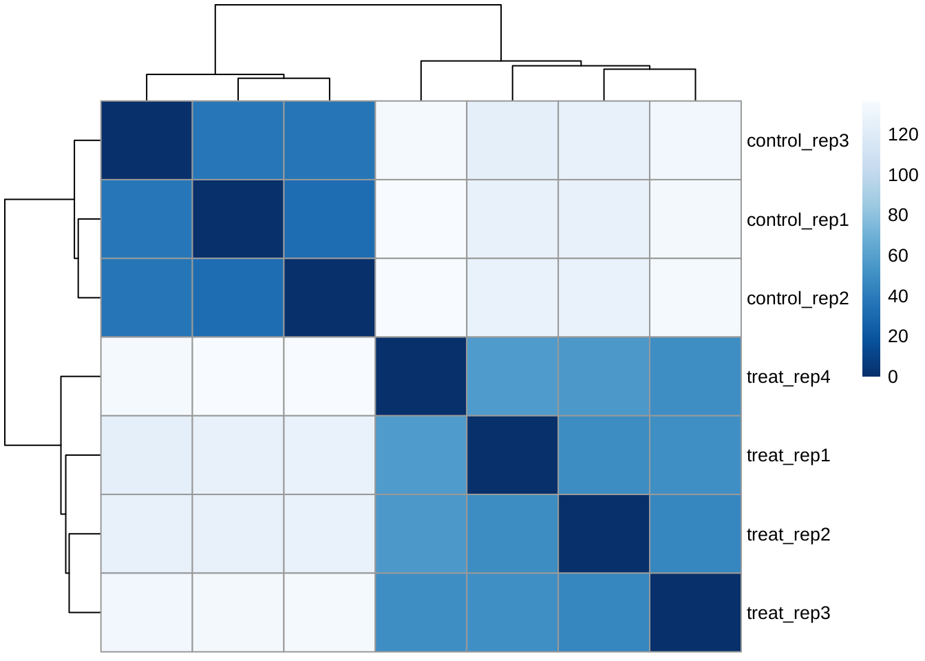
PCA plot (rlog transformed)
Previously we have conducted PCA analysis on samples. Here do PCA plot on genes.
plotPCA(rld)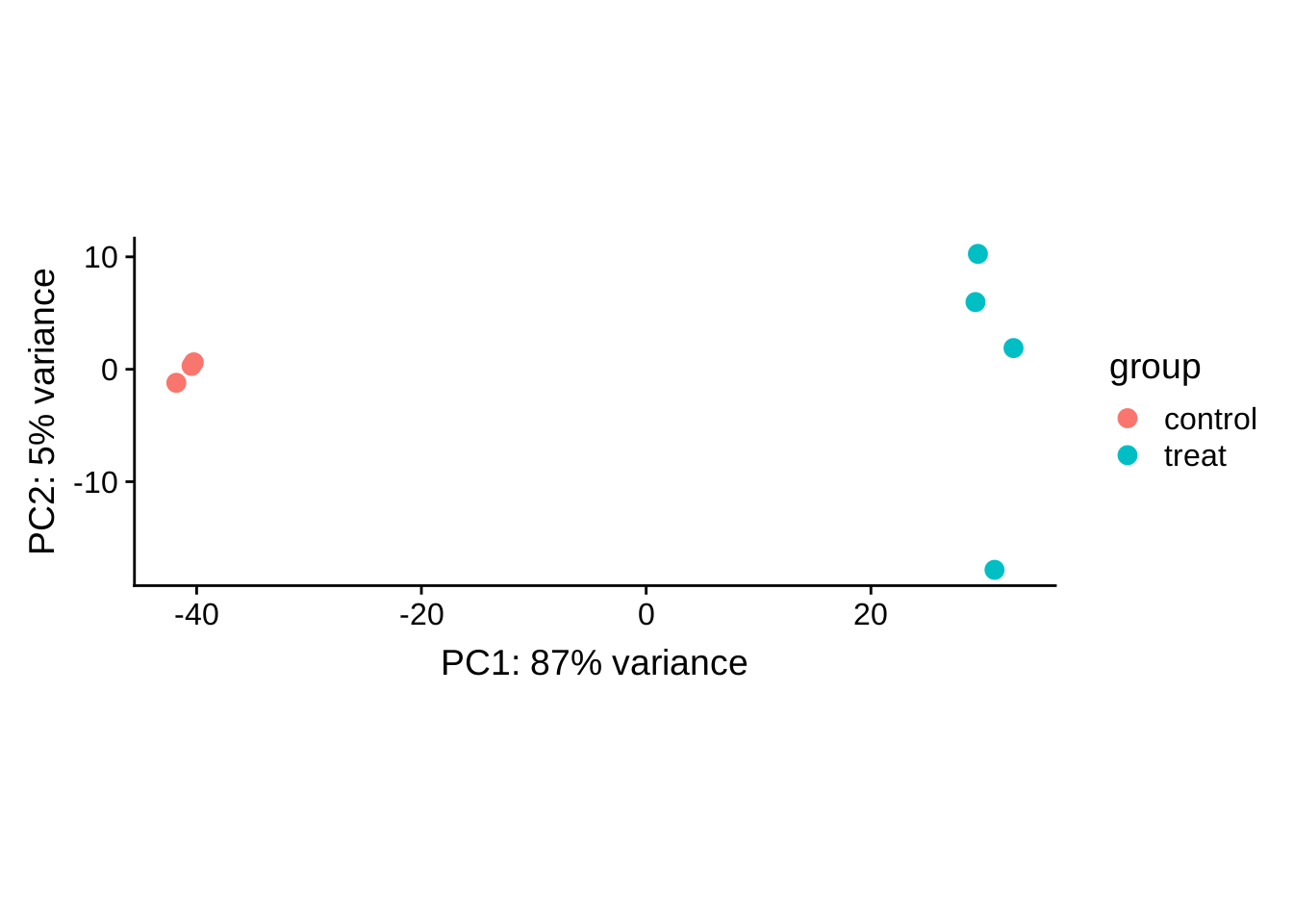
Differential expression analysis
Run the differential expression pipeline.
dds <- DESeq(dds)## estimating size factors## using 'avgTxLength' from assays(dds), correcting for library size## estimating dispersions## gene-wise dispersion estimates## mean-dispersion relationship## final dispersion estimates## fitting model and testingThen build the results table, we use an adjusted p-value cutoff by 0.05.
res <- results(dds, alpha = 0.05)
head(res[order(res$pvalue), ], n = 3)
## log2 fold change (MLE): condition treat vs control
## Wald test p-value: condition treat vs control
## DataFrame with 3 rows and 6 columns
## baseMean log2FoldChange lfcSE
## <numeric> <numeric> <numeric>
## ENSG00000241343 10887.8871376054 -4.06463847625495 0.108594662387474
## ENSG00000185950 7290.71556646402 3.71238174924945 0.103648480871635
## ENSG00000183054 3308.40662655646 5.76746803913769 0.166493932393504
## stat pvalue
## <numeric> <numeric>
## ENSG00000241343 -37.4294499093518 1.29721089573246e-306
## ENSG00000185950 35.8170396520052 5.99696386772001e-281
## ENSG00000183054 34.6407100620727 6.16464222513363e-263
## padj
## <numeric>
## ENSG00000241343 2.4815644435362e-302
## ENSG00000185950 5.73609593947419e-277
## ENSG00000183054 3.93098685889354e-259mcols(res, use.names = TRUE)## DataFrame with 6 rows and 2 columns
## type
## <character>
## baseMean intermediate
## log2FoldChange results
## lfcSE results
## stat results
## pvalue results
## padj results
## description
## <character>
## baseMean mean of normalized counts for all samples
## log2FoldChange log2 fold change (MLE): condition treat vs control
## lfcSE standard error: condition treat vs control
## stat Wald statistic: condition treat vs control
## pvalue Wald test p-value: condition treat vs control
## padj BH adjusted p-valuessummary(res)##
## out of 25001 with nonzero total read count
## adjusted p-value < 0.05
## LFC > 0 (up) : 5536, 22%
## LFC < 0 (down) : 5371, 21%
## outliers [1] : 54, 0.22%
## low counts [2] : 5817, 23%
## (mean count < 1)
## [1] see 'cooksCutoff' argument of ?results
## [2] see 'independentFiltering' argument of ?resultsMA plot
Points are be colored red if the adjusted p value is less than 0.05.
plotMA(res)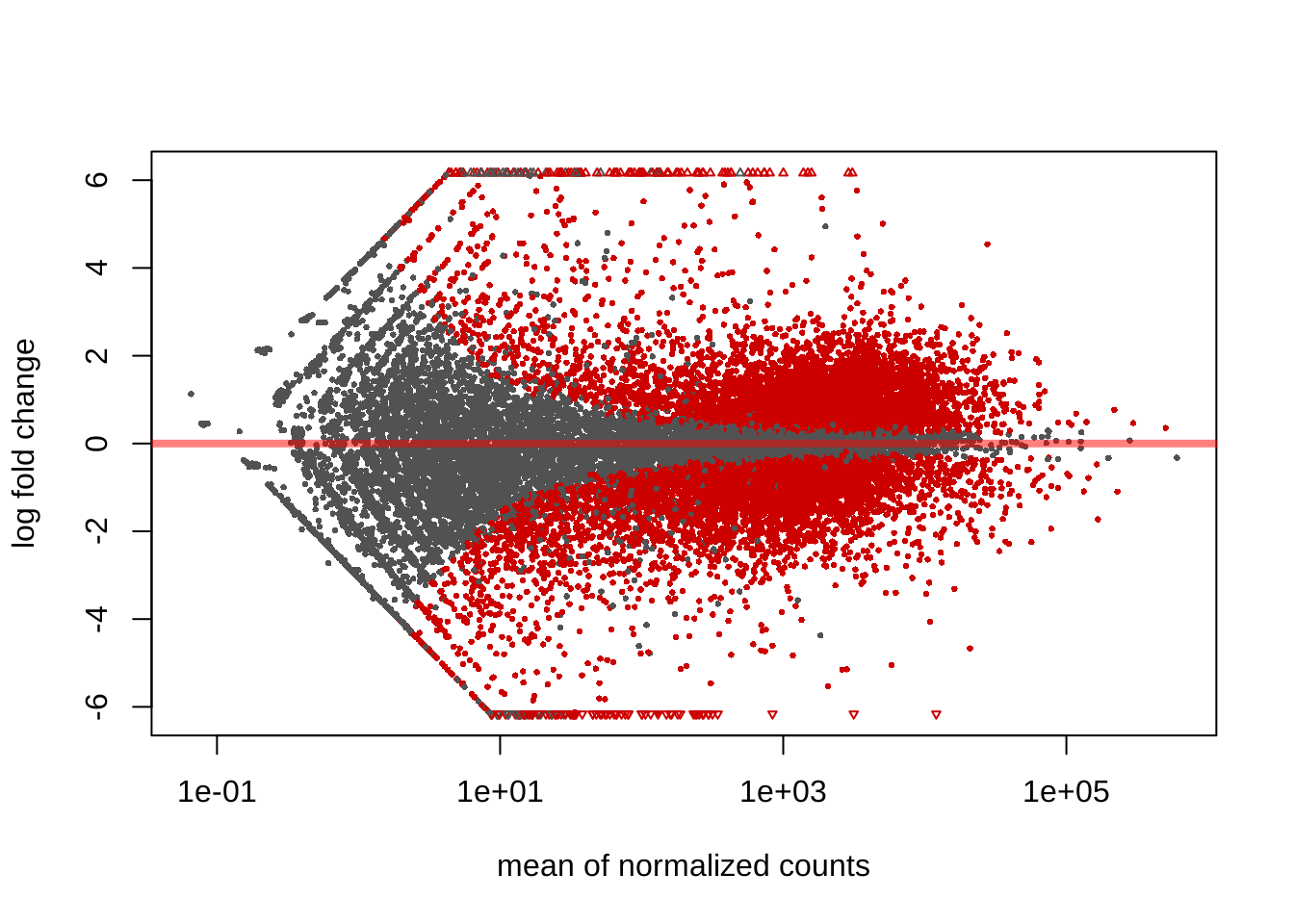
Distribution of p values
hist(res$pvalue[res$baseMean > 1], breaks = 0:20/20,
     col = "grey50", border = "white")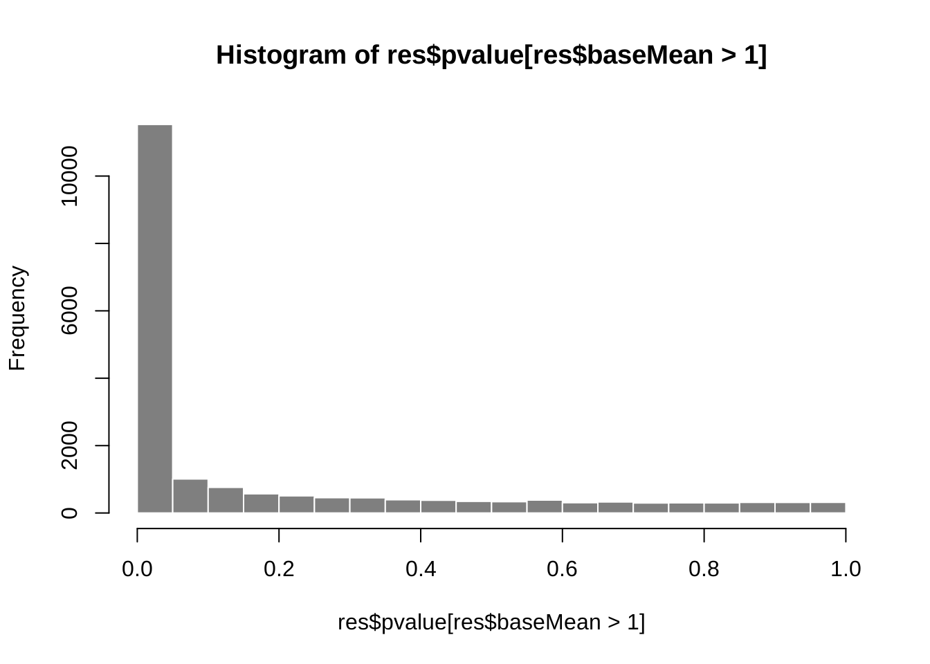
Annotating the gene names
library(AnnotationDbi)
library(org.Hs.eg.db)
res$symbol <- mapIds(org.Hs.eg.db, keys=row.names(res),
    column="SYMBOL", keytype="ENSEMBL", multiVals="first")
## 'select()' returned 1:many mapping between keys and columnsres <- res[, c(ncol(res), 1:(ncol(res)-1))]
head(res[order(res$pvalue),], n = 3)## log2 fold change (MLE): condition treat vs control
## Wald test p-value: condition treat vs control
## DataFrame with 3 rows and 7 columns
## symbol baseMean log2FoldChange
## <character> <numeric> <numeric>
## ENSG00000241343 RPL36A 10887.8871376054 -4.06463847625495
## ENSG00000185950 IRS2 7290.71556646402 3.71238174924945
## ENSG00000183054 RGPD6 3308.40662655646 5.76746803913769
## lfcSE stat pvalue
## <numeric> <numeric> <numeric>
## ENSG00000241343 0.108594662387474 -37.4294499093518 1.29721089573246e-306
## ENSG00000185950 0.103648480871635 35.8170396520052 5.99696386772001e-281
## ENSG00000183054 0.166493932393504 34.6407100620727 6.16464222513363e-263
## padj
## <numeric>
## ENSG00000241343 2.4815644435362e-302
## ENSG00000185950 5.73609593947419e-277
## ENSG00000183054 3.93098685889354e-259Generate a table of differentially expressed genes
We will select the genes that have adjusted p value < 0.05 and order them by their fold change.
Also, since there are a lot of genes differentially expressed, we may be interested in ones that have larger fold change. We will select the ones that have abs(log2foldchange) > 2.
selected <- res[!is.na(res$padj), ]
selected <- selected[selected$padj < 0.05, ]
We selected 10907 out of 25001 genes in the step above.
The following is the distribution of log2foldchange in genes with adjusted p value < 0.05. The yellow bars are ones with fold change < 2, which will be filtered.
hist(sort(selected$log2FoldChange), breaks = 30,
     col = c(rep("white", 14), rep("yellow", 2), rep("white", 14)), xlim = c(-15, 15))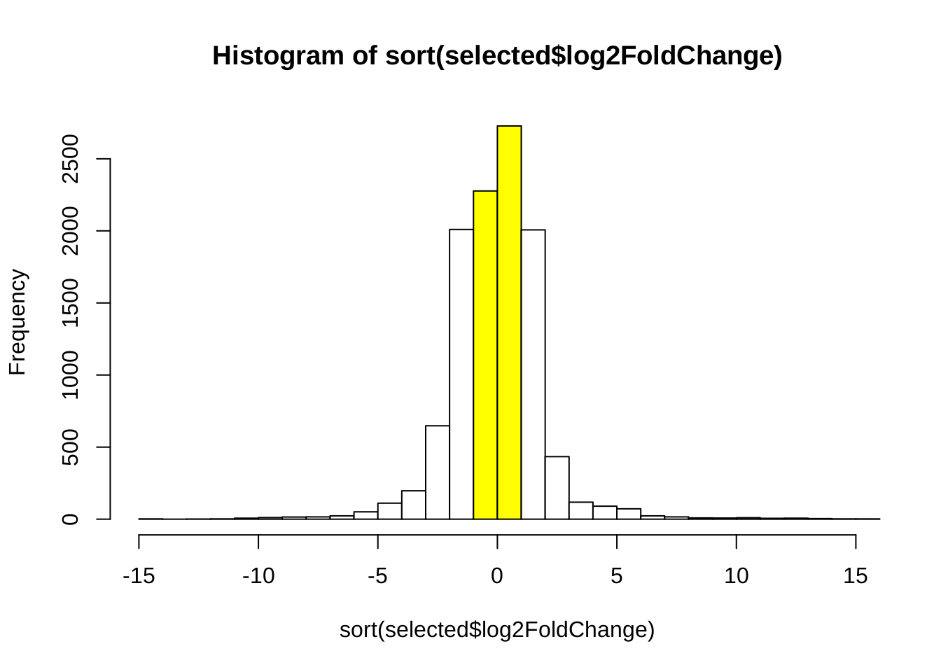
selected <- selected[abs(selected$log2FoldChange) > 2, ]
selected <- selected[order(abs(selected$log2FoldChange), decreasing = TRUE), ]
After filtering by fold change, we finally selected 1885 genes.
Here we generate a table showing the top 100 rows.
selected <- as.data.frame(selected)
selected$log10pvalue <- log10(selected$pvalue)
selected$log10padj <- log10(selected$padj)
selected <- selected[ , c("symbol", "baseMean", "log2FoldChange", "pvalue",
"log10pvalue", "padj", "log10padj")]knitr::kable(selected[1:100,])| symbol | baseMean | log2FoldChange | pvalue | log10pvalue | padj | log10padj | |
|---|---|---|---|---|---|---|---|
| ENSG00000235655 | NA | 3076.70095 | 15.646846 | 0.0000000 | -37.773375 | 0.0000000 | -36.462471 |
| ENSG00000282230 | ADAM9 | 2888.90683 | 15.556043 | 0.0000000 | -27.714462 | 0.0000000 | -26.604766 |
| ENSG00000244398 | NA | 1581.68738 | 14.687067 | 0.0000000 | -34.269128 | 0.0000000 | -33.018822 |
| ENSG00000283485 | NA | 3148.47842 | -14.678216 | 0.0000000 | -45.587733 | 0.0000000 | -44.139802 |
| ENSG00000280830 | ADI1 | 1387.78347 | 14.498522 | 0.0000000 | -33.249811 | 0.0000000 | -32.021942 |
| ENSG00000234851 | NA | 12044.69368 | -14.210605 | 0.0000000 | -83.041873 | 0.0000000 | -80.980266 |
| ENSG00000235043 | NA | 802.98353 | 13.709034 | 0.0000000 | -23.414630 | 0.0000000 | -22.418247 |
| ENSG00000204388 | HSPA1B | 736.70040 | 13.584974 | 0.0000000 | -29.621084 | 0.0000000 | -28.466473 |
| ENSG00000255072 | PIGY | 732.20170 | 13.575567 | 0.0000000 | -29.329213 | 0.0000000 | -28.182312 |
| ENSG00000220842 | NA | 659.11785 | 13.424178 | 0.0000000 | -24.542919 | 0.0000000 | -23.518162 |
| ENSG00000213442 | NA | 428.76061 | 12.804108 | 0.0000000 | -25.512788 | 0.0000000 | -24.461266 |
| ENSG00000283229 | NA | 426.25001 | 12.795152 | 0.0000346 | -4.460787 | 0.0000914 | -4.038870 |
| ENSG00000269378 | NA | 839.92889 | -12.771995 | 0.0000000 | -34.703289 | 0.0000000 | -33.441105 |
| ENSG00000204072 | NA | 405.48635 | 12.723710 | 0.0000000 | -25.790734 | 0.0000000 | -24.730694 |
| ENSG00000283460 | NA | 387.29128 | 12.657692 | 0.0000000 | -25.385382 | 0.0000000 | -24.337678 |
| ENSG00000224472 | TCF19 | 372.57228 | 12.600198 | 0.0000000 | -25.445591 | 0.0000000 | -24.396110 |
| ENSG00000262243 | CES1 | 272.06221 | 12.143572 | 0.0000000 | -21.969075 | 0.0000000 | -21.006050 |
| ENSG00000262327 | AGK | 253.20484 | 12.042178 | 0.0000000 | -15.844717 | 0.0000000 | -15.041713 |
| ENSG00000223654 | FLOT1 | 210.34275 | 11.775529 | 0.0000000 | -22.301366 | 0.0000000 | -21.331193 |
| ENSG00000282735 | KIAA0355 | 175.86971 | 11.518479 | 0.0000000 | -14.421891 | 0.0000000 | -13.658163 |
| ENSG00000233890 | TCF19 | 316.47938 | -11.363763 | 0.0000000 | -27.297103 | 0.0000000 | -26.197231 |
| ENSG00000281289 | LSS | 153.04846 | 11.315626 | 0.0000000 | -20.336677 | 0.0000000 | -19.415177 |
| ENSG00000230043 | NA | 609.14628 | 11.293355 | 0.0000000 | -26.941269 | 0.0000000 | -25.851005 |
| ENSG00000224587 | MDC1 | 297.25882 | -11.273461 | 0.0000000 | -27.013565 | 0.0000000 | -25.921341 |
| ENSG00000173867 | NA | 131.49720 | 11.098474 | 0.0001189 | -3.924739 | 0.0002957 | -3.529176 |
| ENSG00000259132 | NA | 127.78513 | 11.055735 | 0.0000000 | -18.763573 | 0.0000000 | -17.882223 |
| ENSG00000174028 | NA | 245.17011 | -10.995498 | 0.0000000 | -25.743198 | 0.0000000 | -24.685238 |
| ENSG00000257529 | RPL36A-HNRNPH2 | 239.17911 | -10.959490 | 0.0000000 | -25.340422 | 0.0000000 | -24.294740 |
| ENSG00000206492 | GNL1 | 232.70451 | -10.920244 | 0.0000000 | -25.262280 | 0.0000000 | -24.218108 |
| ENSG00000262666 | FAM189B | 102.83438 | 10.744264 | 0.0000000 | -16.952593 | 0.0000000 | -16.121128 |
| ENSG00000223957 | NEU1 | 100.73427 | 10.713972 | 0.0001557 | -3.807719 | 0.0003826 | -3.417262 |
| ENSG00000243251 | NA | 97.08863 | 10.659147 | 0.0000000 | -17.957026 | 0.0000000 | -17.099049 |
| ENSG00000236428 | PPP1R18 | 95.55938 | 10.636517 | 0.0000000 | -18.008242 | 0.0000000 | -17.148460 |
| ENSG00000182774 | RPS17 | 187.07199 | -10.605096 | 0.0000000 | -23.859227 | 0.0000000 | -22.854892 |
| ENSG00000282785 | NA | 1001.73943 | 10.546736 | 0.0000000 | -66.191441 | 0.0000000 | -64.394026 |
| ENSG00000228760 | BAG6 | 159.51923 | -10.375144 | 0.0000000 | -21.825535 | 0.0000000 | -20.865418 |
| ENSG00000283243 | SHANK3 | 149.52376 | -10.281902 | 0.0000000 | -22.369858 | 0.0000000 | -21.397347 |
| ENSG00000281948 | LOC107987423 | 70.89664 | 10.205355 | 0.0000000 | -16.219319 | 0.0000000 | -15.406690 |
| ENSG00000253945 | NA | 67.11174 | 10.128958 | 0.0000000 | -14.367054 | 0.0000000 | -13.604773 |
| ENSG00000283553 | NA | 65.56403 | 10.093708 | 0.0000000 | -15.632485 | 0.0000000 | -14.836633 |
| ENSG00000234196 | ZBTB12 | 130.40189 | -10.084548 | 0.0000000 | -20.816319 | 0.0000000 | -19.882324 |
| ENSG00000263020 | NA | 63.82464 | 10.062020 | 0.0000000 | -13.527041 | 0.0000000 | -12.788400 |
| ENSG00000280852 | LOC653653 | 249.37149 | 10.029893 | 0.0000000 | -39.067065 | 0.0000000 | -37.730819 |
| ENSG00000203812 | HIST2H2AA3 | 59.38863 | 9.950450 | 0.0000000 | -15.155185 | 0.0000000 | -14.375487 |
| ENSG00000234648 | NA | 115.78445 | -9.913479 | 0.0000000 | -20.235413 | 0.0000000 | -19.316180 |
| ENSG00000234964 | NA | 106.16769 | -9.787543 | 0.0000000 | -18.517243 | 0.0000000 | -17.642408 |
| ENSG00000275300 | MCCC2 | 82.00449 | 9.779681 | 0.0000000 | -14.223894 | 0.0000000 | -13.466835 |
| ENSG00000277641 | WNT3 | 100.41017 | -9.707385 | 0.0075049 | -2.124653 | 0.0146514 | -1.834120 |
| ENSG00000236418 | HLA-DQA1 | 100.16776 | -9.703914 | 0.0075264 | -2.123415 | 0.0146888 | -1.833014 |
| ENSG00000223618 | VPS52 | 48.40785 | 9.656625 | 0.0003463 | -3.460597 | 0.0008188 | -3.086830 |
| ENSG00000267059 | NA | 254.83601 | -9.617788 | 0.0000000 | -20.436333 | 0.0000000 | -19.513124 |
| ENSG00000244563 | NA | 40.14673 | 9.385623 | 0.0000000 | -12.715493 | 0.0000000 | -11.996903 |
| ENSG00000114790 | ARHGEF26 | 80.13651 | -9.382221 | 0.0000000 | -17.757058 | 0.0000000 | -16.905580 |
| ENSG00000258677 | NA | 76.59470 | -9.317170 | 0.0000000 | -18.036393 | 0.0000000 | -17.175624 |
| ENSG00000124205 | EDN3 | 268.99825 | 9.313617 | 0.0000000 | -31.109931 | 0.0000000 | -29.927551 |
| ENSG00000267534 | S1PR2 | 37.28580 | 9.280728 | 0.0000000 | -13.338519 | 0.0000000 | -12.605930 |
| ENSG00000237580 | NA | 36.99971 | 9.269904 | 0.0000000 | -12.009517 | 0.0000000 | -11.313263 |
| ENSG00000273398 | NA | 72.06234 | -9.228464 | 0.0000000 | -16.994242 | 0.0000000 | -16.161542 |
| ENSG00000281742 | MCCC2 | 66.61644 | -9.115579 | 0.0000000 | -16.854846 | 0.0000000 | -16.026143 |
| ENSG00000166783 | MARF1 | 65.98720 | -9.101793 | 0.0000000 | -14.286921 | 0.0000000 | -13.527128 |
| ENSG00000272780 | NA | 63.89816 | -9.055748 | 0.0000000 | -16.919849 | 0.0000000 | -16.088691 |
| ENSG00000278573 | NA | 31.76068 | 9.048547 | 0.0006120 | -3.213241 | 0.0013989 | -2.854199 |
| ENSG00000283149 | NA | 59.69974 | -8.958003 | 0.0000000 | -16.044382 | 0.0000000 | -15.236883 |
| ENSG00000262633 | NA | 56.52239 | -8.878874 | 0.0000000 | -16.128320 | 0.0000000 | -15.318190 |
| ENSG00000227317 | DDAH2 | 55.09922 | -8.841597 | 0.0148923 | -1.827037 | 0.0276110 | -1.558917 |
| ENSG00000152086 | TUBA3E | 27.38916 | 8.835309 | 0.0000000 | -11.428499 | 0.0000000 | -10.748410 |
| ENSG00000256968 | NA | 26.74882 | 8.801180 | 0.0000000 | -10.765160 | 0.0000000 | -10.108654 |
| ENSG00000267697 | LUZP6 | 26.26094 | 8.774552 | 0.0005166 | -3.286876 | 0.0011933 | -2.923244 |
| ENSG00000235692 | PFDN6 | 50.95973 | -8.728953 | 0.0162194 | -1.789966 | 0.0298458 | -1.525117 |
| ENSG00000231878 | NA | 25.29156 | 8.721717 | 0.0000000 | -10.994723 | 0.0000000 | -10.328010 |
| ENSG00000282684 | ZC3H3 | 47.88194 | -8.639698 | 0.0000000 | -14.959121 | 0.0000000 | -14.184857 |
| ENSG00000167711 | SERPINF2 | 45.21632 | -8.557066 | 0.0000000 | -11.932473 | 0.0000000 | -11.239254 |
| ENSG00000280158 | NA | 45.15382 | -8.554864 | 0.0000000 | -14.299419 | 0.0000000 | -13.538842 |
| ENSG00000242361 | HLA-DMA | 21.74032 | 8.499219 | 0.0000000 | -9.344540 | 0.0000000 | -8.733071 |
| ENSG00000186076 | NA | 565.21314 | 8.420632 | 0.0000973 | -4.011969 | 0.0002439 | -3.612836 |
| ENSG00000273707 | CDKN1C | 151.56088 | 8.327926 | 0.0000227 | -4.643106 | 0.0000611 | -4.213688 |
| ENSG00000185641 | NA | 190.70288 | 8.313943 | 0.0000000 | -12.647322 | 0.0000000 | -11.929681 |
| ENSG00000230336 | POU5F1 | 18.56966 | 8.274299 | 0.0246028 | -1.609016 | 0.0437611 | -1.358912 |
| ENSG00000277086 | MTMR10 | 34.41780 | -8.162631 | 0.0000000 | -12.826292 | 0.0000000 | -12.105678 |
| ENSG00000263809 | NA | 33.67410 | -8.131452 | 0.0000000 | -12.245246 | 0.0000000 | -11.541252 |
| ENSG00000230143 | FLOT1 | 33.62465 | -8.129907 | 0.0000000 | -12.652086 | 0.0000000 | -11.934208 |
| ENSG00000180581 | NA | 33.31416 | -8.115694 | 0.0254239 | -1.594758 | 0.0451042 | -1.345783 |
| ENSG00000263620 | NA | 32.91314 | -8.098944 | 0.0000000 | -12.897451 | 0.0000000 | -12.174565 |
| ENSG00000267001 | NA | 32.14571 | -8.064379 | 0.0000000 | -12.932927 | 0.0000000 | -12.209080 |
| ENSG00000280571 | NA | 52.23861 | -8.052881 | 0.0000000 | -11.591445 | 0.0000000 | -10.907535 |
| ENSG00000253816 | NA | 31.31488 | -8.025978 | 0.0000000 | -12.587029 | 0.0000000 | -11.871162 |
| ENSG00000217733 | NA | 84.65976 | 7.998947 | 0.0000000 | -17.195517 | 0.0000000 | -16.356595 |
| ENSG00000277044 | OPRL1 | 15.28371 | 7.992178 | 0.0013284 | -2.876658 | 0.0029110 | -2.535957 |
| ENSG00000277278 | HERC2 | 29.00972 | -7.916123 | 0.0000000 | -12.342978 | 0.0000000 | -11.634831 |
| ENSG00000270136 | MINOS1-NBL1 | 179.64712 | -7.913475 | 0.0000000 | -10.336730 | 0.0000000 | -9.694401 |
| ENSG00000232569 | GABBR1 | 13.98351 | 7.863862 | 0.0000000 | -8.680086 | 0.0000000 | -8.089629 |
| ENSG00000275326 | NOSTRIN | 30.40018 | 7.826545 | 0.0000001 | -6.996009 | 0.0000003 | -6.471235 |
| ENSG00000277150 | F8A3 | 26.93577 | -7.809527 | 0.0000000 | -11.650948 | 0.0000000 | -10.965390 |
| ENSG00000171532 | NEUROD2 | 244.57296 | 7.796966 | 0.0000000 | -41.285240 | 0.0000000 | -39.916278 |
| ENSG00000136244 | IL6 | 25.65669 | -7.734676 | 0.0000000 | -10.470953 | 0.0000000 | -9.824219 |
| ENSG00000227222 | DHX16 | 24.77538 | -7.689310 | 0.0000000 | -11.076587 | 0.0000000 | -10.407232 |
| ENSG00000273003 | ARL2-SNX15 | 24.74304 | -7.686421 | 0.0000000 | -10.523655 | 0.0000000 | -9.875005 |
| ENSG00000227402 | SLC39A7 | 88.92664 | 7.680142 | 0.0084928 | -2.070952 | 0.0164157 | -1.784740 |
| ENSG00000120675 | DNAJC15 | 135.07129 | 7.627673 | 0.0000000 | -39.815275 | 0.0000000 | -38.465018 |
| ENSG00000234218 | MICB | 23.05480 | -7.585511 | 0.0000000 | -10.570884 | 0.0000000 | -9.920917 |
Gene clustering
Clustering of all selected genes by expression level (rlog transformed)
library(genefilter)##
## Attaching package: 'genefilter'## The following objects are masked from 'package:matrixStats':
##
## rowSds, rowVarsmat <- assay(rld)[rownames(selected), ]
anno <- as.data.frame(colData(rld)[, c("condition", "sample_name")])
pheatmap(mat, annotation_col = anno, show_rownames = FALSE,
main = "Heatmap of rlog-transformed gene expression levels")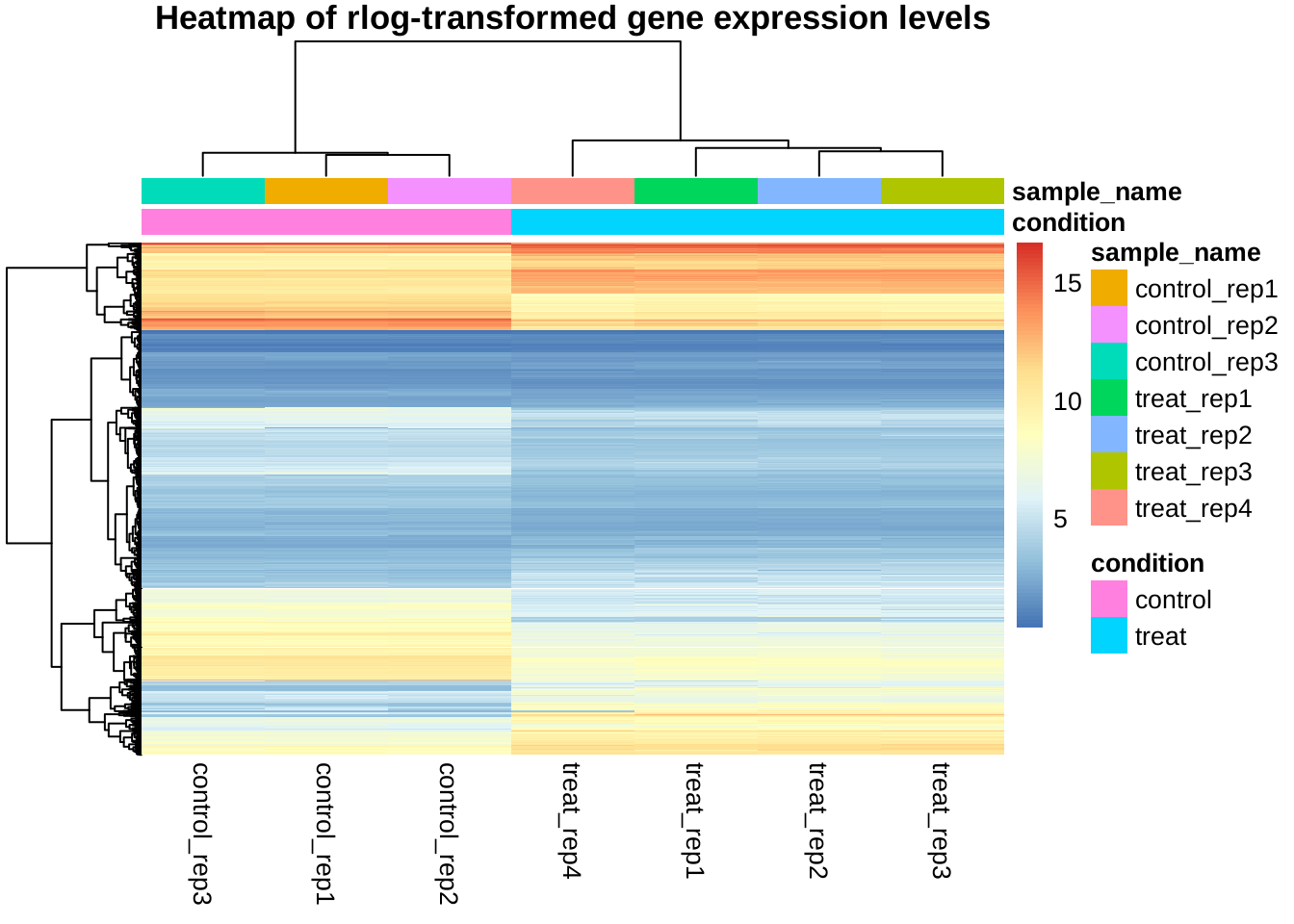
Clustering of all selected genes by relative expression levels across samples
Instead of absolute expression strength, the following plot uses the amount by which each gene deviates in a specific sample from the gene’s average across all samples.
The trees on top shows the clustering by samples, the trees on left shows the clustering by genes. It can be shown that the control and treat samples are clearly separated and the genes may be roughly divided into two clusters (up-regulated and down-regulated).
mat <- mat - rowMeans(mat)
pheatmap(mat, annotation_col = anno, show_rownames = FALSE,
         main = "Heatmap of relative rlog-transformed values across samples")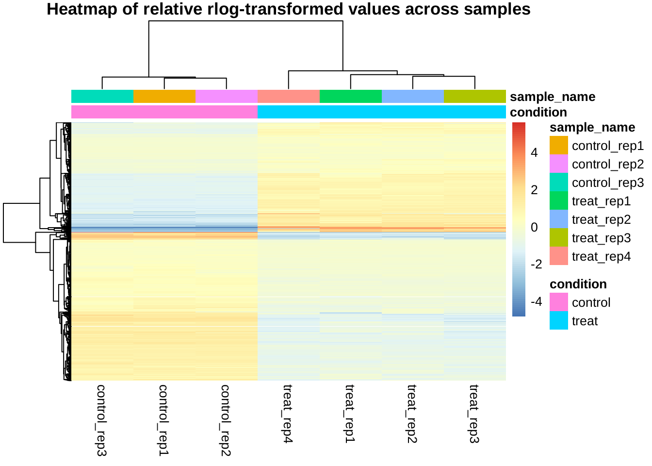
Clustering of genes with the highest variance across samples
Here we select the 30 genes with the highest variance of expression values across samples.
library(genefilter)
topVarGenes <- head(order(rowVars(assay(rld)), decreasing = TRUE), 30)
mat <- assay(rld)[topVarGenes, ]
mat <- mat[rownames(mat) %in% rownames(selected), ]
mat <- mat - rowMeans(mat)
anno <- as.data.frame(colData(rld)[, c("condition", "sample_name")])
pheatmap(mat, annotation_col = anno,
         main = "Heatmap of relative rlog-transformed values across samples")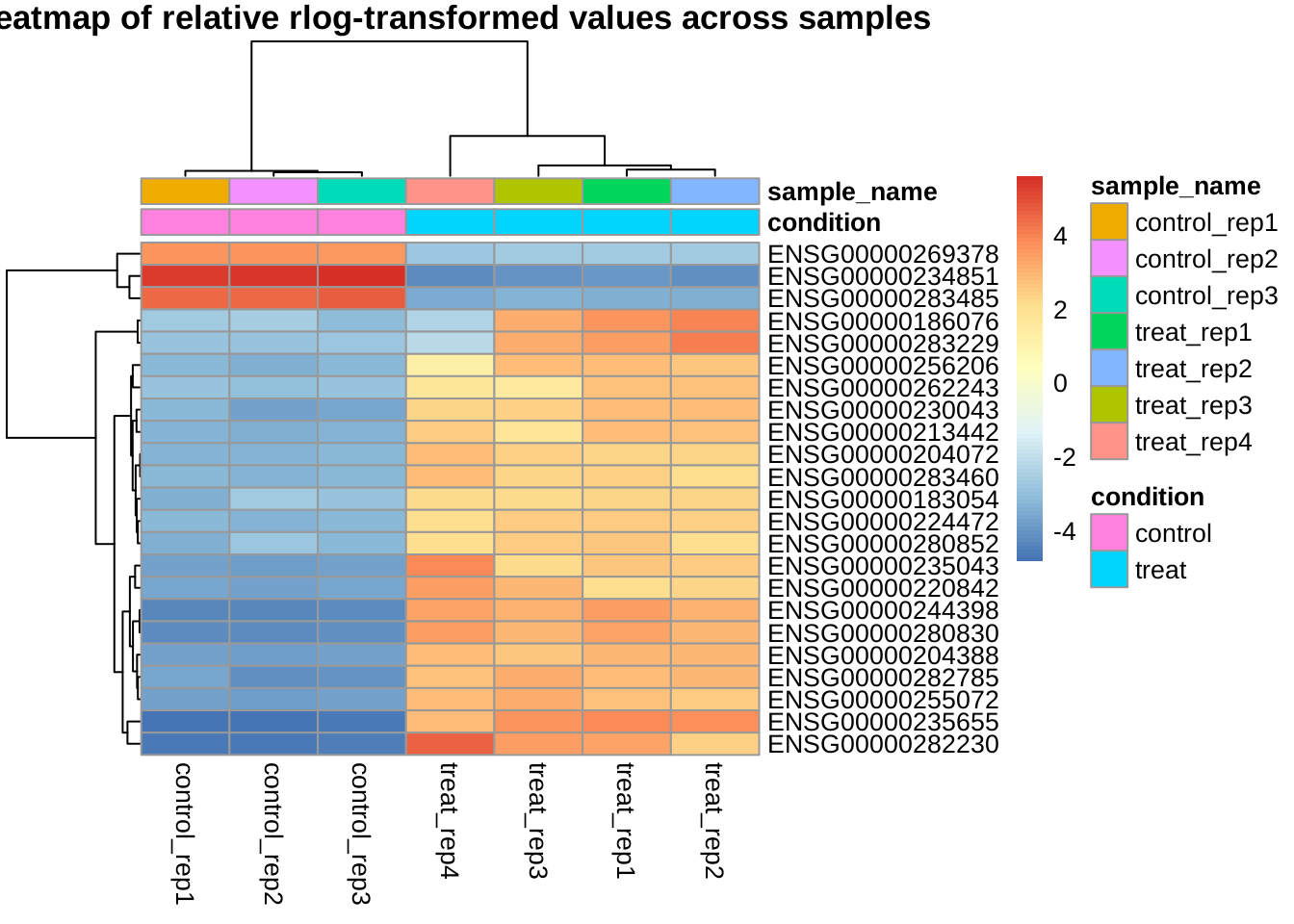
PCA plot of genes
We will use rlog-transformed values. The following is a PCA plot of all selected genes.
library(ggfortify)
autoplot(prcomp(assay(rld)[rownames(assay(rld)) %in% rownames(selected), ]), size = 1, alpha = 0.8)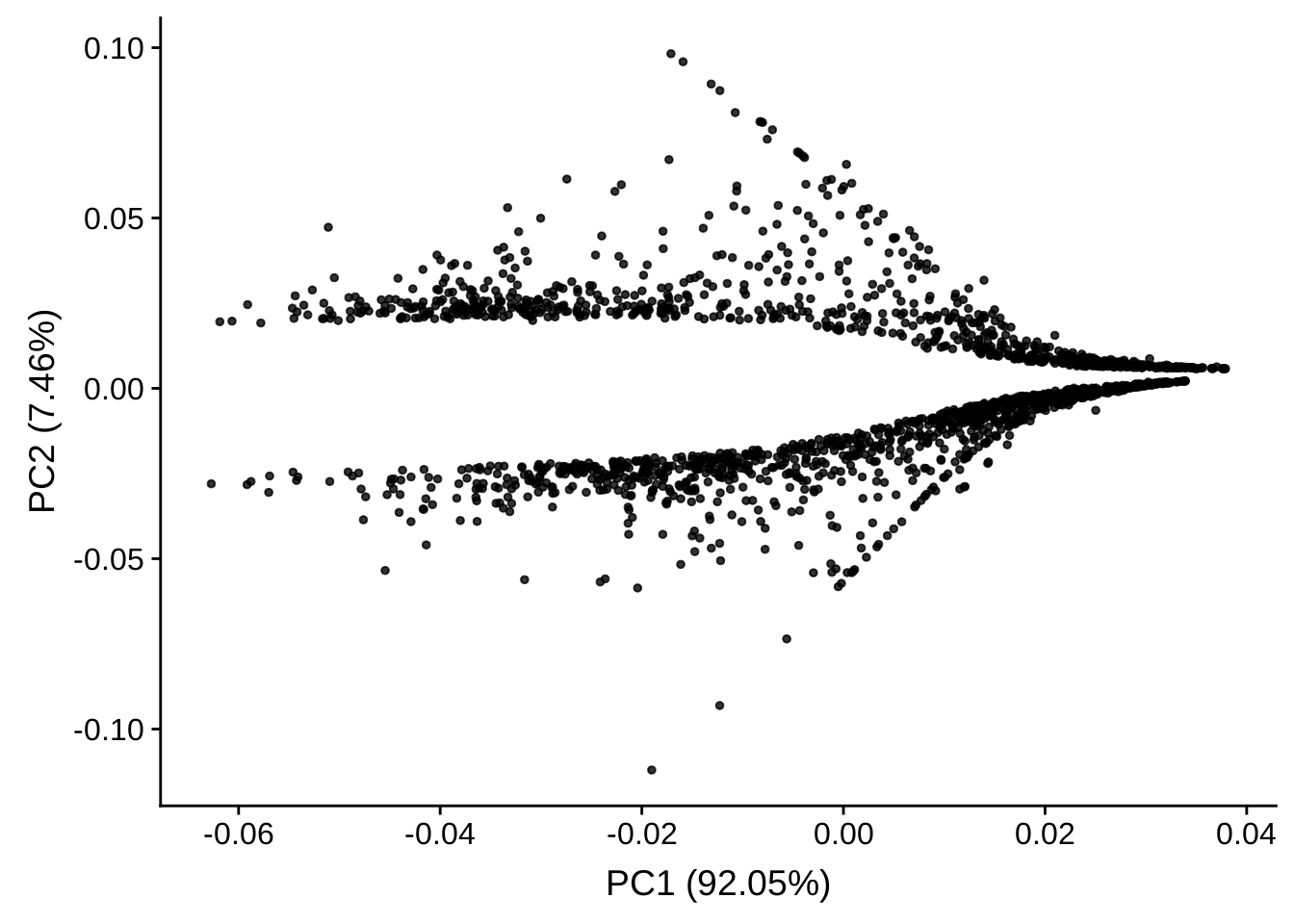
It is clear that the genes can be separated by two parts by the second dimension. If we plot all the genes like the following, it will be clear for us that the second dimension aligns with the foldchange – since we have filtered the genes with low foldchange. Thus the two clusters are up-regulated genes and down-regulated genes.
autoplot(prcomp(assay(rld)[rownames(assay(rld)), ]), size = 1, alpha = 0.8)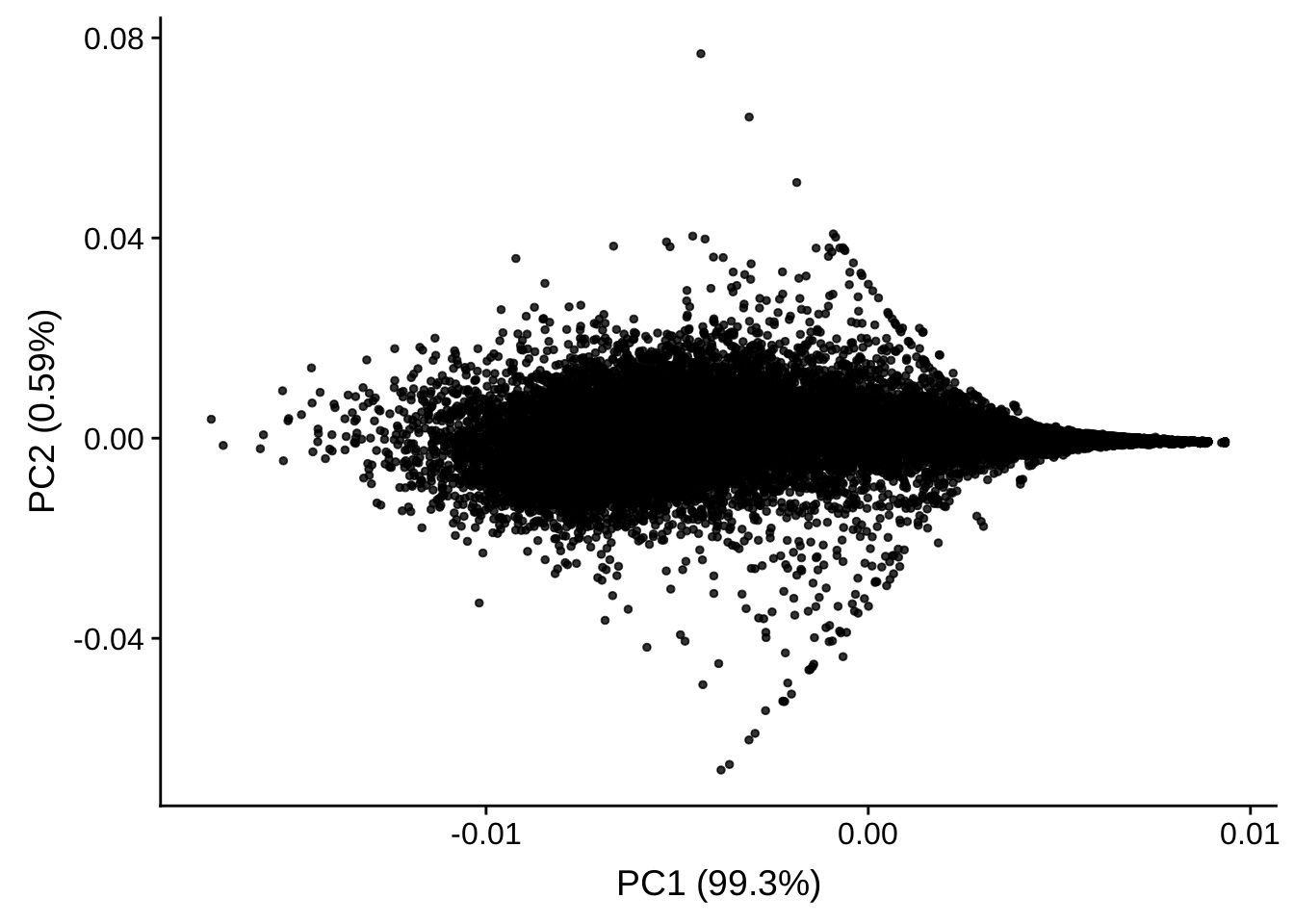
PCA plot of genes with high variance
Again, we select the genes with the highest variance across samples:
topVarGenes <- head(order(rowVars(assay(rld)), decreasing = TRUE), 50)
tmp <- assay(rld)[topVarGenes, ]
tmp <- tmp[rownames(tmp) %in% rownames(selected), ]
autoplot(prcomp(tmp))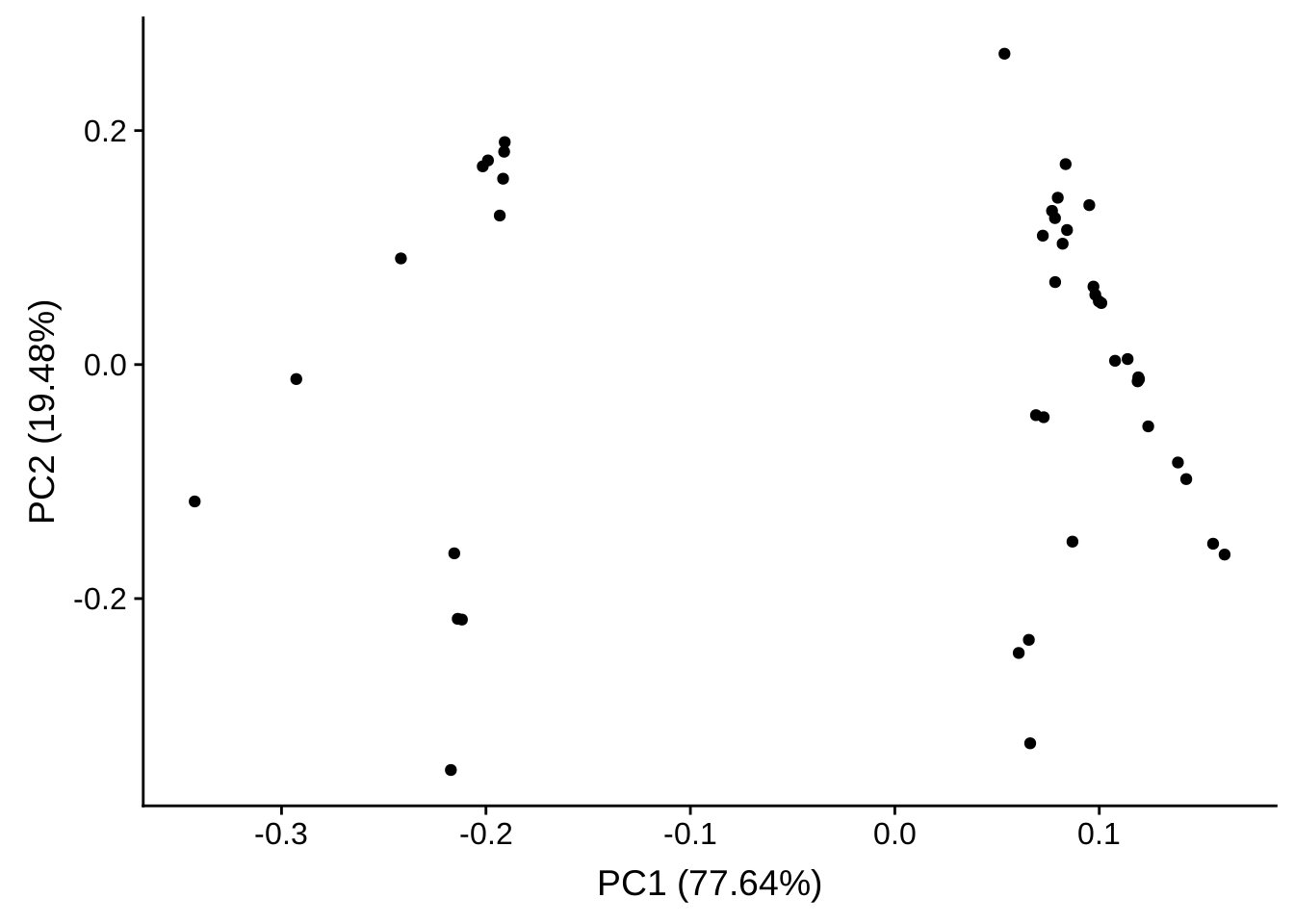
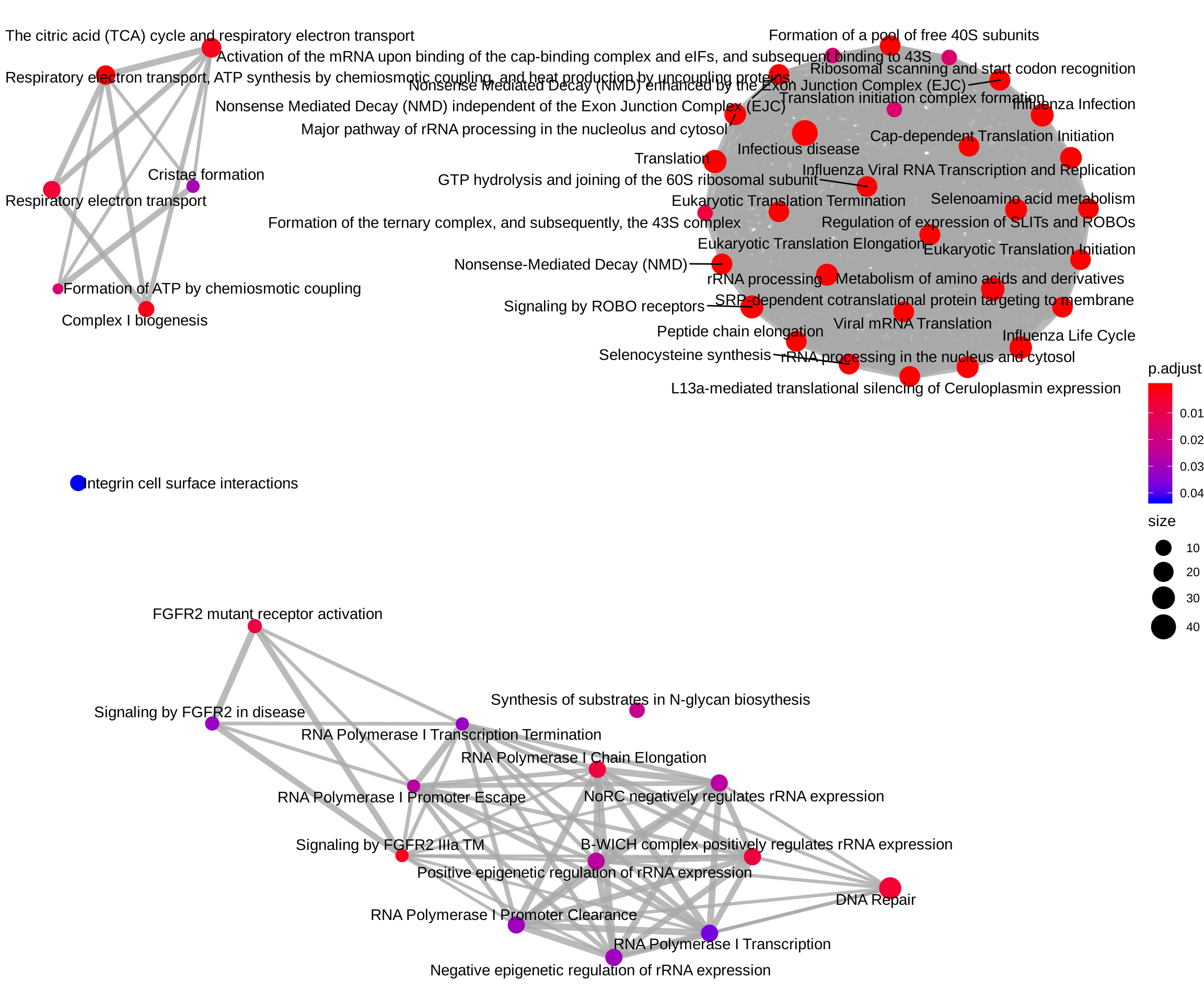
Pathway analysis
The package ReactomePA offers the possibility to test enrichment of specific pathways using the free, open-source, curated and peer reviewed pathway Reactome pathway database.
library(ReactomePA)
entrez_ids <- mapIds(org.Hs.eg.db, keys = rownames(res),
                     column = "ENTREZID", keytype = "ENSEMBL", multiVals = "first")
## 'select()' returned 1:many mapping between keys and columnsentrez_ids <- entrez_ids[rownames(selected)]
entrez_ids <- entrez_ids[!is.na(entrez_ids)]
reactome_enrich <- enrichPathway(gene = entrez_ids, organism = "human", readable = TRUE)Then we visualize the enriched terms.
barplot(reactome_enrich, showCategory = 25)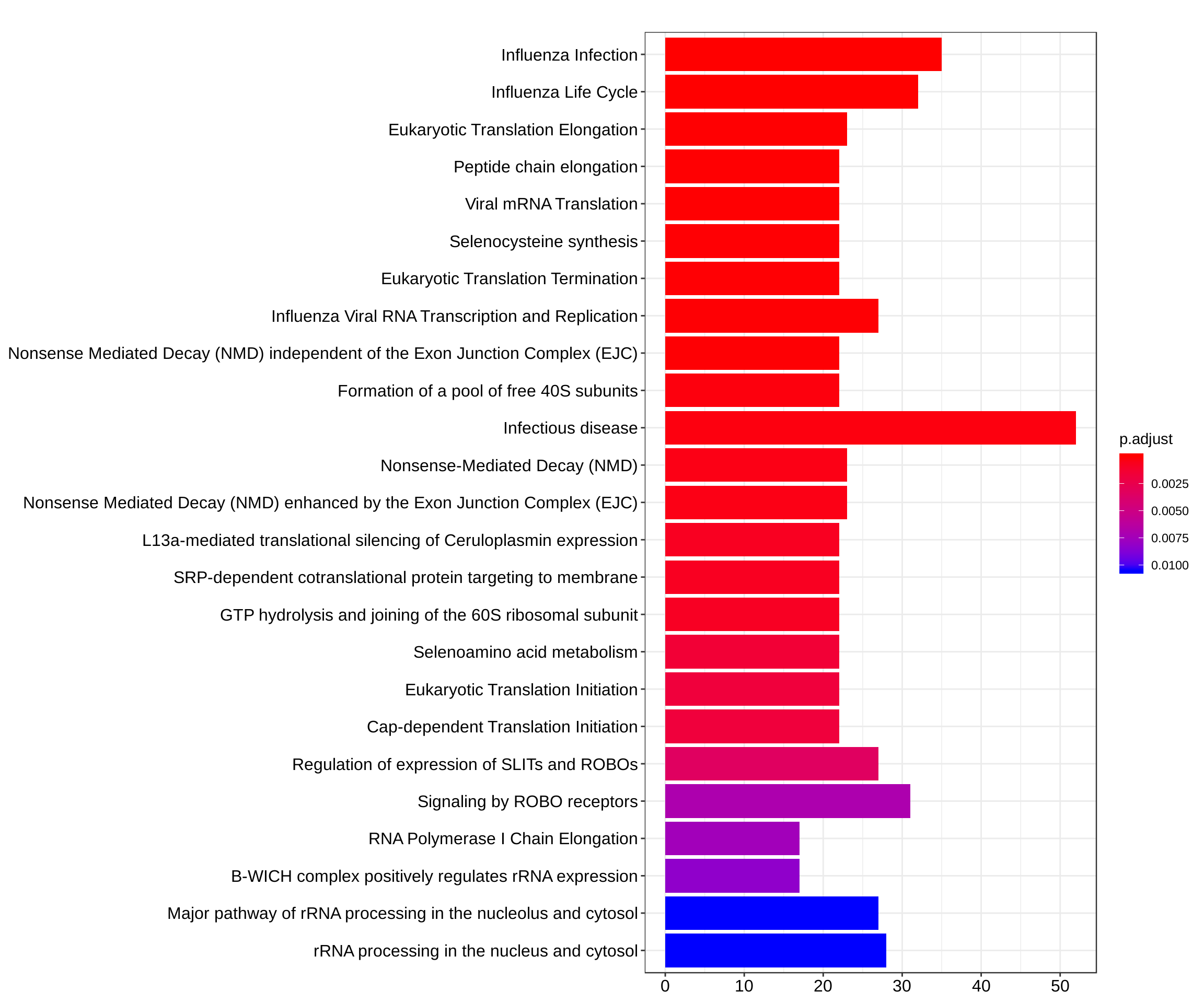
dotplot(reactome_enrich, showCategory = 25)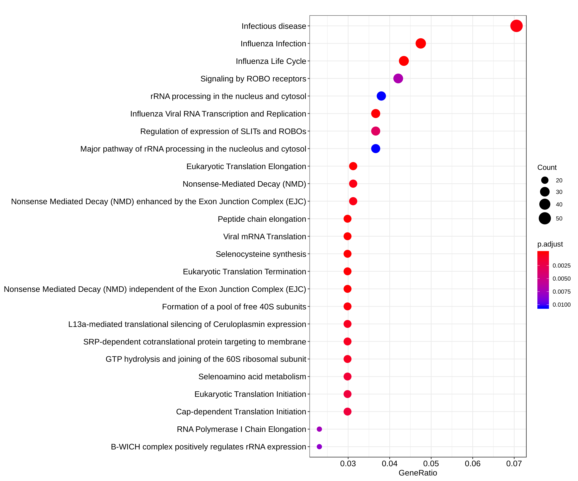
ReactomePA::emapplot(reactome_enrich, showCategory = Inf)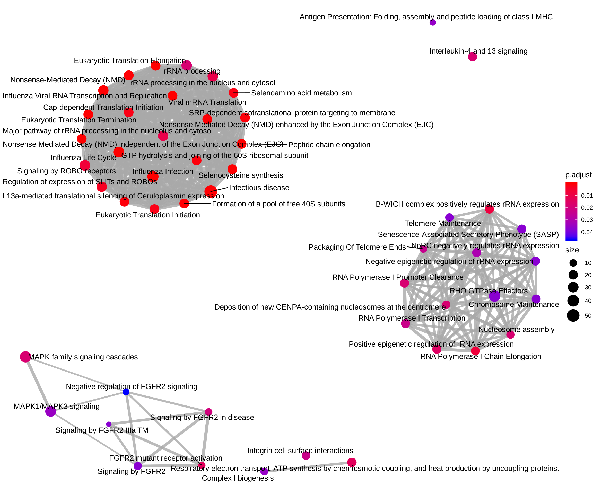
Pathway analysis of up-regulated genes
up_regulated <- selected[selected$log2FoldChange > 0, ]
up_regulated <- up_regulated[rownames(up_regulated) %in% names(entrez_ids), ]
tryCatch(
    ReactomePA::emapplot(
        enrichPathway(gene = entrez_ids[rownames(up_regulated)], organism = "human"),
        showCategory = Inf),
    error = function(e) print(e$message)
)
## [1] "no enriched term found..."However we do not have any term enriched given the up-regulated genes.
Pathway analysis of down-regulated genes
down_regulated <- selected[selected$log2FoldChange < 0, ]
down_regulated <- down_regulated[rownames(down_regulated) %in% names(entrez_ids), ]
ReactomePA::emapplot(
    enrichPathway(gene = entrez_ids[rownames(down_regulated)], organism = "human"),
    showCategory = Inf)