Microarray Data Analysis
Jialin Ma
October 17, 2018
Load Packages
suppressPackageStartupMessages({
    library(here)
    library(oligo)
})
Load the dataset
- GSM651311 Keratinocytes, untreated 24h, rep1
- GSM651316 Keratinocytes, DEX-treated 24h, rep1
- GSM651321 Keratinocytes, untreated 24h, rep2
- GSM651326 Keratinocytes, DEX-treated 24h, rep2
dataset <- read.celfiles(list.files(here("data/microarray"), full.names = TRUE))## Loading required package: pd.hg.u95av2## Loading required package: RSQLite## Loading required package: DBI## Platform design info loaded.## Reading in : /home/jialin/Courses/code6150/data/microarray/GSM651309.CEL.gz
## Reading in : /home/jialin/Courses/code6150/data/microarray/GSM651310.CEL.gz
## Reading in : /home/jialin/Courses/code6150/data/microarray/GSM651311.CEL.gz
## Reading in : /home/jialin/Courses/code6150/data/microarray/GSM651312.CEL.gz
## Reading in : /home/jialin/Courses/code6150/data/microarray/GSM651313.CEL.gz
## Reading in : /home/jialin/Courses/code6150/data/microarray/GSM651314.CEL.gz
## Reading in : /home/jialin/Courses/code6150/data/microarray/GSM651315.CEL.gz
## Reading in : /home/jialin/Courses/code6150/data/microarray/GSM651316.CEL.gz
## Reading in : /home/jialin/Courses/code6150/data/microarray/GSM651317.CEL.gz
## Reading in : /home/jialin/Courses/code6150/data/microarray/GSM651318.CEL.gz
## Reading in : /home/jialin/Courses/code6150/data/microarray/GSM651319.CEL.gz
## Reading in : /home/jialin/Courses/code6150/data/microarray/GSM651320.CEL.gz
## Reading in : /home/jialin/Courses/code6150/data/microarray/GSM651321.CEL.gz
## Reading in : /home/jialin/Courses/code6150/data/microarray/GSM651322.CEL.gz
## Reading in : /home/jialin/Courses/code6150/data/microarray/GSM651323.CEL.gz
## Reading in : /home/jialin/Courses/code6150/data/microarray/GSM651324.CEL.gz
## Reading in : /home/jialin/Courses/code6150/data/microarray/GSM651325.CEL.gz
## Reading in : /home/jialin/Courses/code6150/data/microarray/GSM651326.CEL.gz
## Reading in : /home/jialin/Courses/code6150/data/microarray/GSM651327.CEL.gz
## Reading in : /home/jialin/Courses/code6150/data/microarray/GSM651328.CEL.gz#dataset <- dataset[, c(paste0(c("GSM651310", "GSM651320", "GSM651315", "GSM651325"), ".CEL.gz"))]
dataset <- dataset[, c(paste0(c("GSM651311", "GSM651321", "GSM651316", "GSM651326"), ".CEL.gz"))]
sampleNames(dataset) <- c("control_rep1", "control_rep2", "treat_rep1", "treat_rep2")
pData(dataset)$group <- c("control", "control", "treat", "treat")
dataset## ExpressionFeatureSet (storageMode: lockedEnvironment)
## assayData: 409600 features, 4 samples
## element names: exprs
## protocolData
## rowNames: control_rep1 control_rep2 treat_rep1 treat_rep2
## varLabels: exprs dates
## varMetadata: labelDescription channel
## phenoData
## rowNames: control_rep1 control_rep2 treat_rep1 treat_rep2
## varLabels: index group
## varMetadata: labelDescription channel
## featureData: none
## experimentData: use 'experimentData(object)'
## Annotation: pd.hg.u95av2Quality control
Boxplot
boxplot(dataset, target = "core")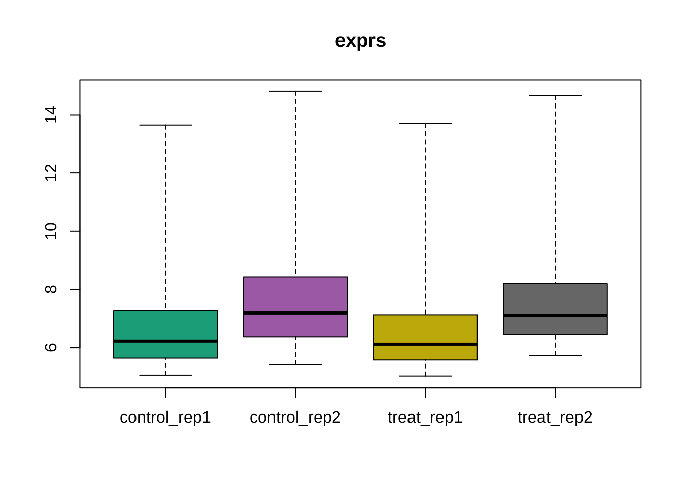
MA plot
oligo::MAplot(dataset, pairs = TRUE, ylim = c(-1, 1))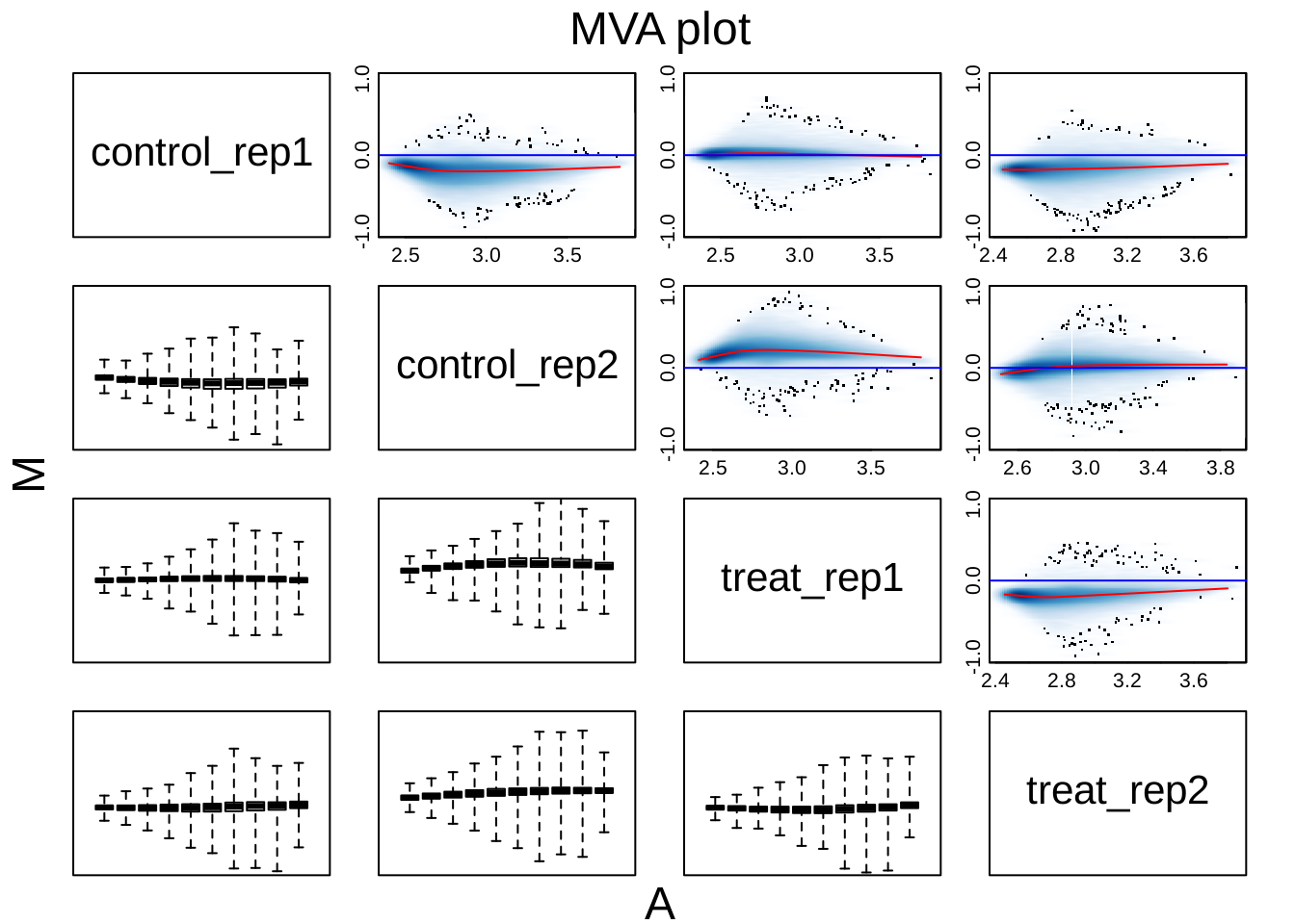
Quality report of the raw data
The following will generate a quality report of the raw microarray data in docs/microarray_qualitymetrics directory.
library(arrayQualityMetrics)
arrayQualityMetrics(expressionset = dataset,
    outdir = "docs/microarray_qualitymetrics",
    force = TRUE, do.logtransform = TRUE,
    intgroup = c("group"))
RMA
The RMA method proceeds with background subtraction, normalization and summarization using a deconvolution method for background correction, quantile normalization and the RMA (robust multichip average) algorithm for summarization.
edata <- oligo::rma(dataset)## Background correcting
## Normalizing
## Calculating Expressionedata## ExpressionSet (storageMode: lockedEnvironment)
## assayData: 12625 features, 4 samples
## element names: exprs
## protocolData
## rowNames: control_rep1 control_rep2 treat_rep1 treat_rep2
## varLabels: exprs dates
## varMetadata: labelDescription channel
## phenoData
## rowNames: control_rep1 control_rep2 treat_rep1 treat_rep2
## varLabels: index group
## varMetadata: labelDescription channel
## featureData: none
## experimentData: use 'experimentData(object)'
## Annotation: pd.hg.u95av2Access the quality after normalization
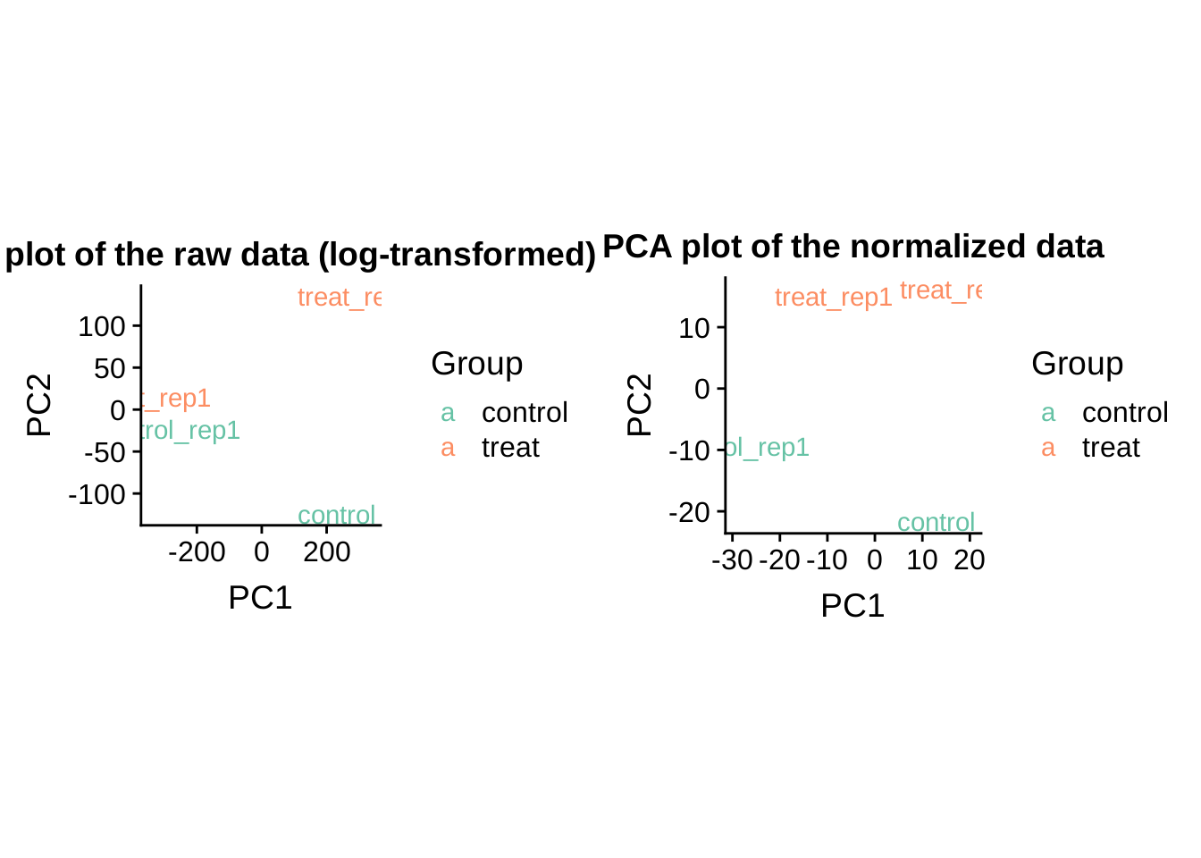
PCA plot before and after normalization
library(ggplot2)
library(cowplot)
##
## Attaching package: 'cowplot'## The following object is masked from 'package:ggplot2':
##
## ggsaveplot_grid(
local({
PCA_raw <- prcomp(t(log2(exprs(dataset))), scale = FALSE)
dataGG <- data.frame(PC1 = PCA_raw$x[,1], PC2 = PCA_raw$x[,2],
Group = pData(dataset)$group)
qplot(PC1, PC2, data = dataGG, color = Group,
main = "PCA plot of the raw data (log-transformed)", asp = 1.0, geom = "text",
label = sampleNames(dataset)) + scale_colour_brewer(palette = "Set2")
}),
local({
PCA <- prcomp(t(exprs(edata)), scale = FALSE)
dataGG <- data.frame(PC1 = PCA$x[,1], PC2 = PCA$x[,2],
Group = pData(dataset)$group)
qplot(PC1, PC2, data = dataGG, color = Group,
main = "PCA plot of the normalized data", asp = 1.0, geom = "text",
label = sampleNames(edata)) +
scale_colour_brewer(palette = "Set2")
})
)
Boxplot before and after normalization
par(mfrow = c(1,2))
boxplot(dataset)
boxplot(edata)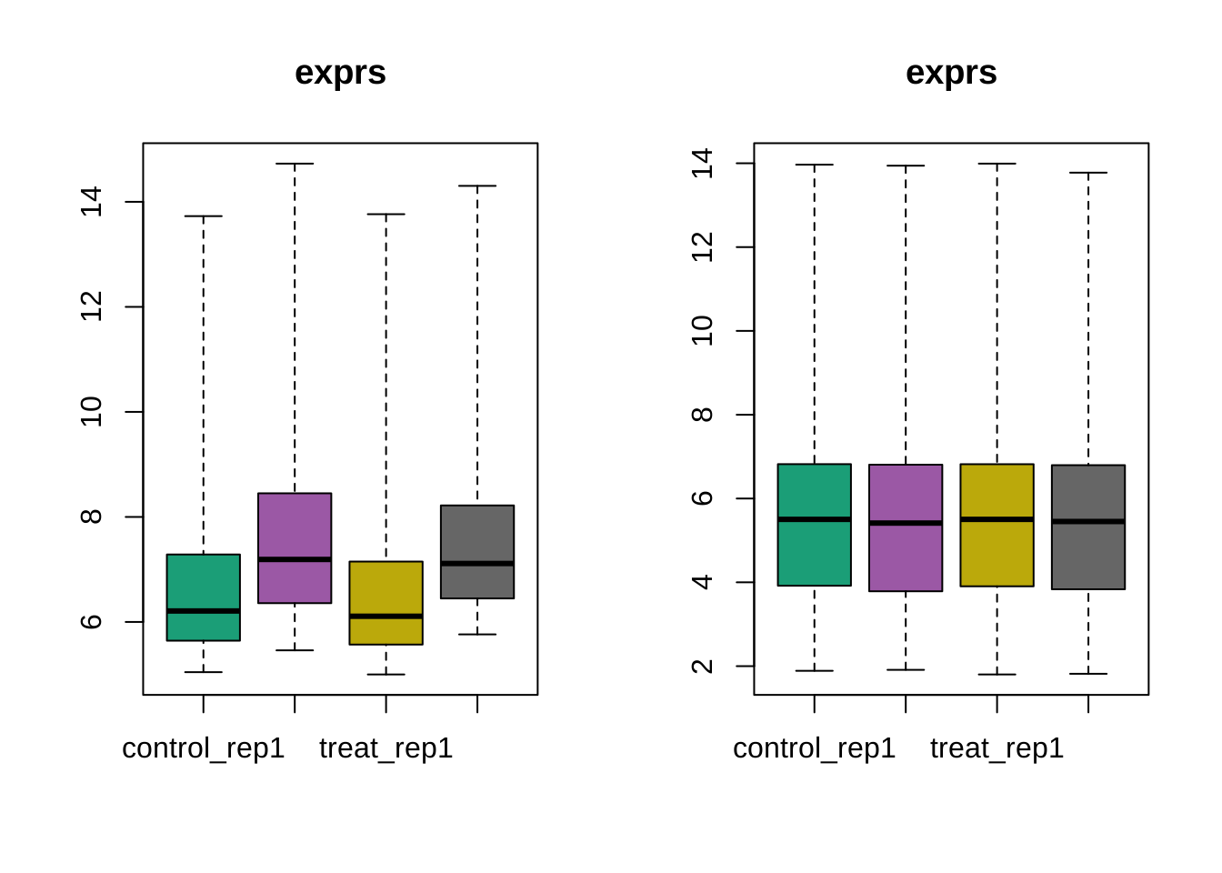
par(mfrow = c(1,1))MA plot after normalization
oligo::MAplot(edata, pairs = TRUE, ylim = c(-1, 1))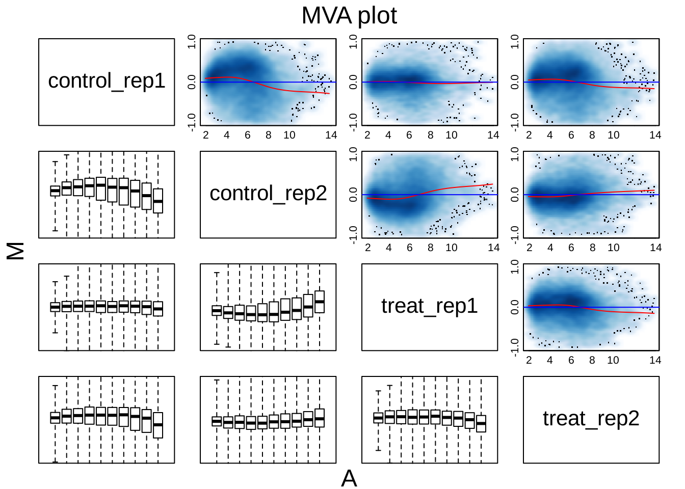
Heatmap with sample-to-sample distance after normalization
It can not provide too much information for us since the number of samples is limited.
library(RColorBrewer)
library(pheatmap)
dists <- as.matrix(dist(t(exprs(edata)), method = "manhattan"))
diag(dists) <- NA
hmcol <- colorRampPalette(rev(brewer.pal(9, "PuOr")))(255)
pheatmap(dists, col = rev(hmcol), clustering_distance_rows = "manhattan",
                    clustering_distance_cols = "manhattan")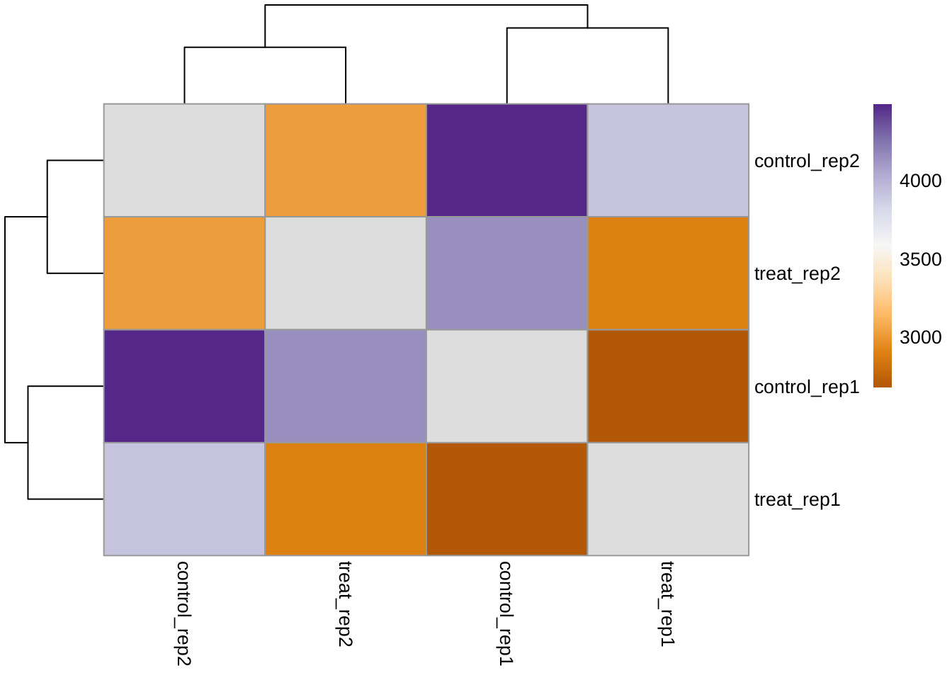
Filter based on intensity
Microarray data commonly show a large number of probes in the background intensity range. They also do not change much across arrays. Hence they combine a low variance with a low intensity. We want to filter these results as they may contribute to false positive results in the differential expression analysis. The bars represent the distribution of median intensities, the red vertical line represents the threshold value. If more than two samples of a gene have intensities larger than the threshold value, the gene will be kept.
edata_medians <- rowMedians(exprs(edata))
hist_res <- hist(edata_medians, 100, col="#e7efd8", freq = FALSE,
                 main = "Histogram of the median intensities",
                 xlab = "Median intensities")
emp_mu <- hist_res$breaks[which.max(hist_res$density)]
emp_sd <- mad(edata_medians)/2
prop_cental <- 0.50
lines(sort(edata_medians),
      prop_cental*dnorm(sort(edata_medians), mean = emp_mu, sd = emp_sd),
    col = "grey10", lwd = 3)

#cut_val <- 0.05 / prop_cental
thresh_median <- qnorm(0.05 / prop_cental, emp_mu, emp_sd)
abline(v = thresh_median, lwd = 4, col = "red")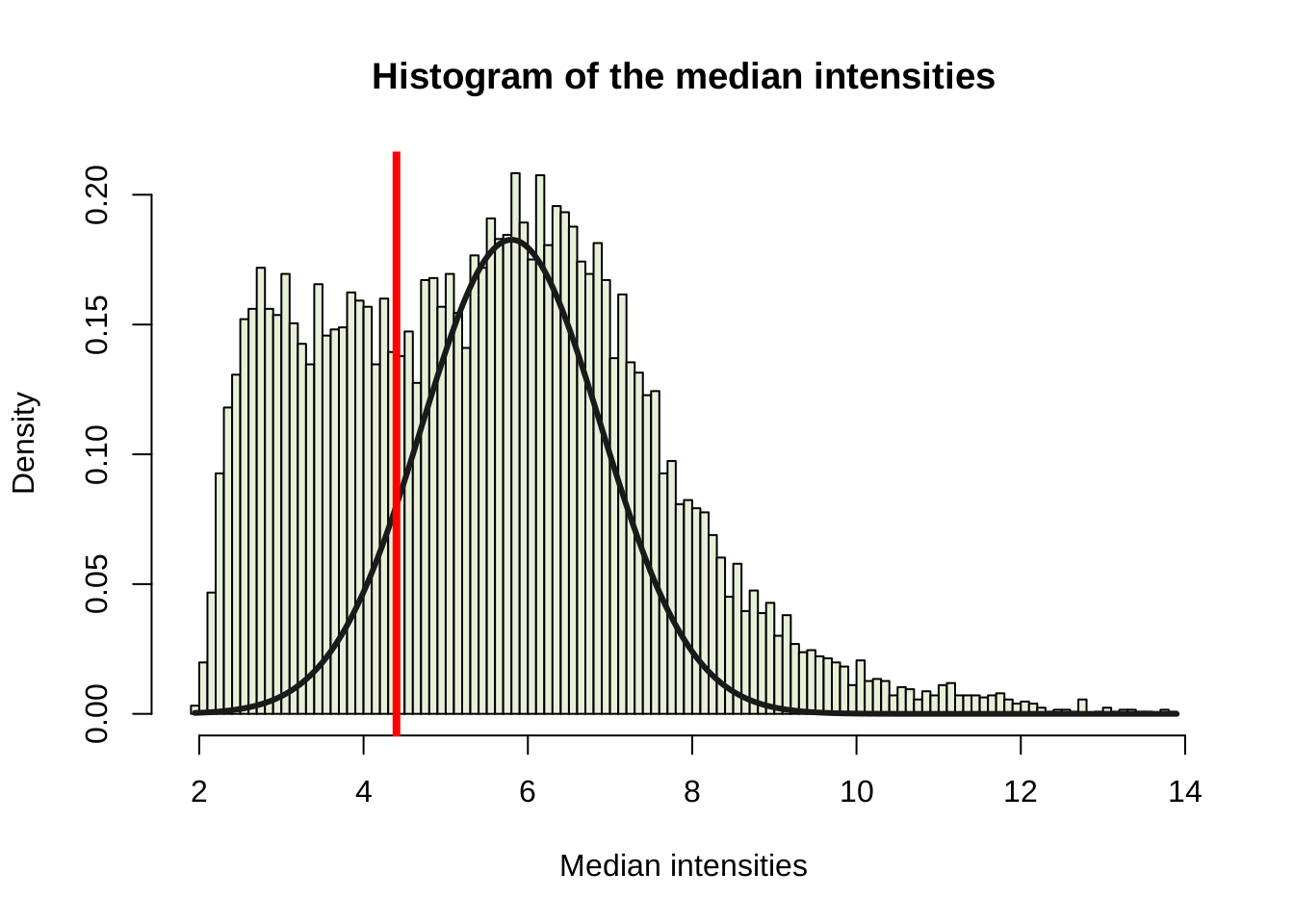
samples_cutoff <- 2
idx_thresh_median <- apply(exprs(edata), 1, function(x){
                   sum(x > thresh_median) >= samples_cutoff})
table(idx_thresh_median)
## idx_thresh_median
## FALSE TRUE
## 4060 8565edata <- subset(edata, idx_thresh_median)Identification of differentially expressed genes
Create a design matrix. We will also consider the batch effects between replicates in order to remove them.
library(limma)##
## Attaching package: 'limma'## The following object is masked from 'package:oligo':
##
## backgroundCorrect## The following object is masked from 'package:BiocGenerics':
##
## plotMAf <- factor(c("control", "control", "treat", "treat"))
batch <- factor(c("rep1", "rep2", "rep1", "rep2"))
design <- model.matrix(~ 0 + f + batch)
colnames(design)## [1] "fcontrol" "ftreat" "batchrep2"colnames(design) <- c("control", "treat", "batch")
design## control treat batch
## 1 1 0 0
## 2 1 0 1
## 3 0 1 0
## 4 0 1 1
## attr(,"assign")
## [1] 1 1 2
## attr(,"contrasts")
## attr(,"contrasts")$f
## [1] "contr.treatment"
##
## attr(,"contrasts")$batch
## [1] "contr.treatment"We can fit the linear model, define appropriate contrast to test the hypothesis on treatment effect and compute the moderated t–statistics by calling the eBayes function.
data.fit <- lmFit(exprs(edata), design)
head(data.fit$coefficients)
## control treat batch
## 100_g_at 7.797102 8.130695 -0.2555991
## 1000_at 7.593515 7.814241 0.1087141
## 1002_f_at 4.612296 4.664025 -0.1417638
## 1003_s_at 6.091525 6.084982 -0.2208167
## 1004_at 5.848525 5.979026 -0.1795733
## 1005_at 8.166263 9.442745 -0.3113774contrast.matrix <- makeContrasts(treat-control,levels=design)
data.fit.con <- contrasts.fit(data.fit,contrast.matrix)
data.fit.eb <- eBayes(data.fit.con)Volcano plot to show the distribution of fold change and p value.
volcanoplot(data.fit.eb,highlight=10)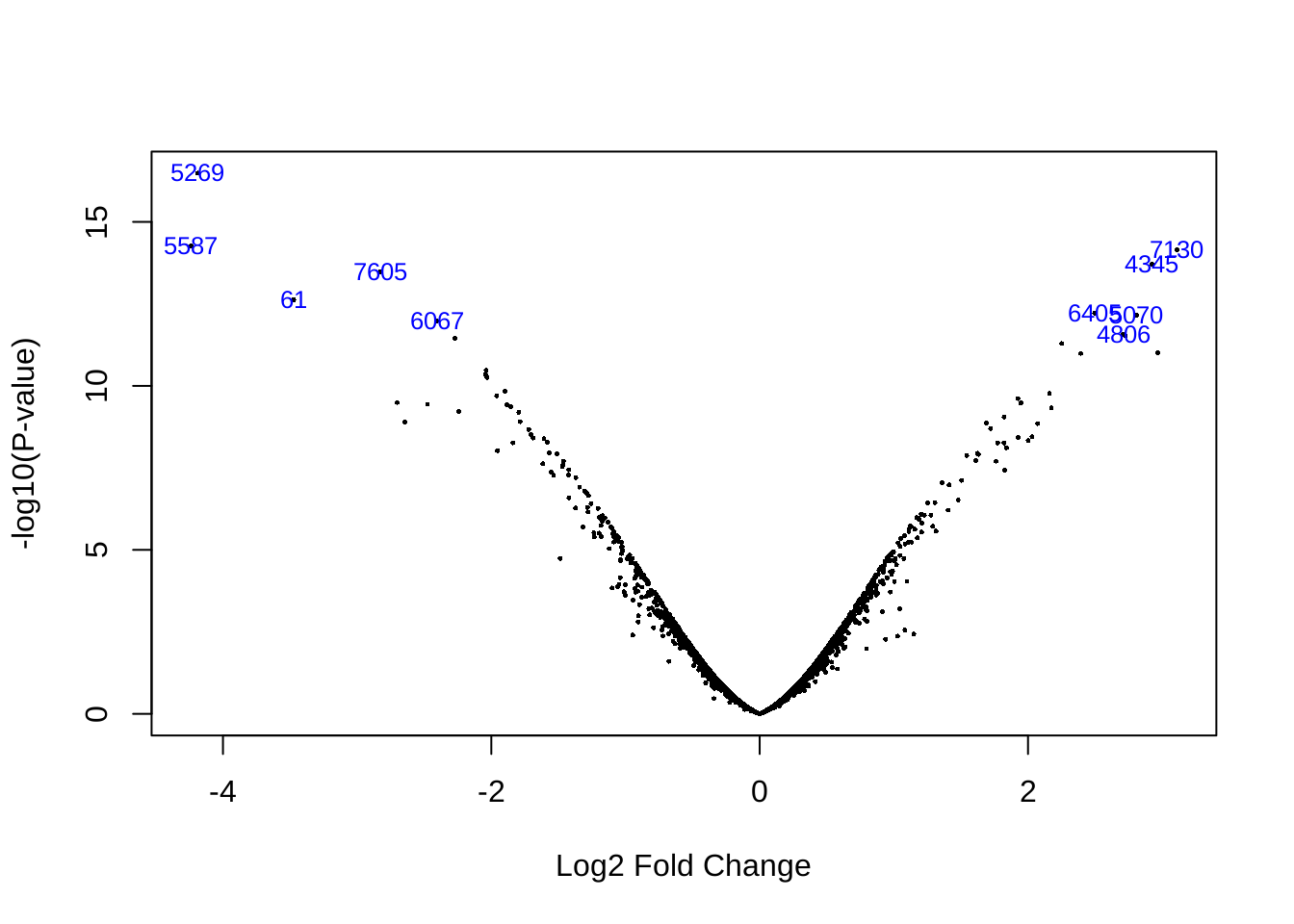
Then we sort the results by their absolute t-statistics.
top <- topTable(data.fit.eb, number = Inf)
head(top)
## logFC AveExpr t P.Value adj.P.Val B
## 37989_at -4.187867 5.058882 -21.61960 3.275846e-17 2.805762e-13 28.37765
## 38428_at -4.238118 5.624551 -17.23860 5.383859e-15 2.020411e-11 23.91131
## 40522_at 3.109750 8.149514 17.02754 7.076745e-15 2.020411e-11 23.66414
## 36629_at 2.923410 7.890901 16.27198 1.929437e-14 4.131408e-11 22.75146
## 41193_at -2.827488 6.189725 -15.87952 3.299633e-14 5.652271e-11 22.25952
## 1081_at -3.472805 7.263600 -14.50306 2.373227e-13 3.387781e-10 20.43040Check how many results can we get if we use a p value cutoff by 0.001 or an adjusted p value cutoff by 0.05.
table(top$adj.P.Val < 0.05)##
## FALSE TRUE
## 8117 448table(top$P.Value < 0.001)##
## FALSE TRUE
## 8205 360We would like to visualize the distribution of p value with a histogram.
hist(top$P.Value, col = brewer.pal(3, name = "Set2")[1], breaks = 100,
      main = "Control vs Treatment of DEX", xlab = "p-values")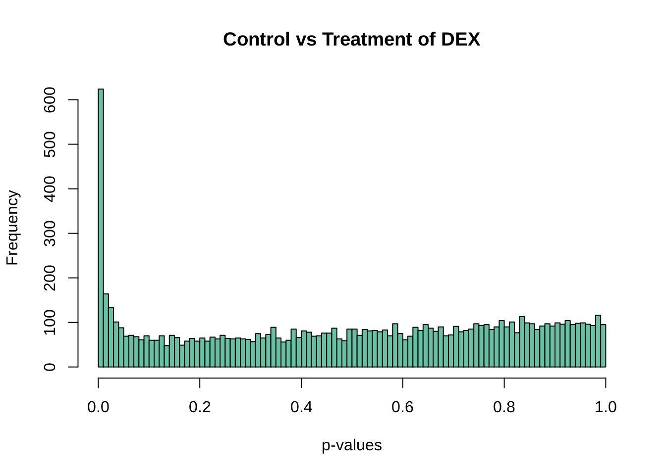
Annotating genes
We need to annotate the gene names by the probe IDs.
suppressPackageStartupMessages({
    library(hgu95av2.db)
})
get_symbol <- function(probeid) {
    ans <- mapIds(hgu95av2.db::hgu95av2.db,
                  keys = probeid, keytype = "PROBEID", column = "SYMBOL", multiVals = "first")
    unname(ans)
}
get_genename <- function(probeid) {
    ans <- mapIds(hgu95av2.db::hgu95av2.db,
                  keys = probeid, keytype = "PROBEID", column = "GENENAME", multiVals = "first")
    unname(ans)
}
top$symbol <- get_symbol(rownames(top))
## 'select()' returned 1:many mapping between keys and columnstop$gene_name <- get_genename(rownames(top))## 'select()' returned 1:many mapping between keys and columnsGenerate a table of differentially expressed genes
We will use a cutoff of adjusted p value by 0.05.
selected <- top[, c("symbol", "gene_name", "logFC", "P.Value", "adj.P.Val")]
#top <- cbind(data.frame(probeID = rownames(top), stringsAsFactors = FALSE), top)
#rownames(top) <- NULL
selected <- selected[selected$adj.P.Val < 0.05,]
nrow(selected)
## [1] 448We will only show the first 100 genes.
knitr::kable(selected[1:100,])| symbol | gene_name | logFC | P.Value | adj.P.Val | |
|---|---|---|---|---|---|
| 37989_at | PTHLH | parathyroid hormone like hormone | -4.187867 | 0.0e+00 | 0.0000000 |
| 38428_at | MMP1 | matrix metallopeptidase 1 | -4.238118 | 0.0e+00 | 0.0000000 |
| 40522_at | GLUL | glutamate-ammonia ligase | 3.109750 | 0.0e+00 | 0.0000000 |
| 36629_at | TSC22D3 | TSC22 domain family member 3 | 2.923410 | 0.0e+00 | 0.0000000 |
| 41193_at | DUSP6 | dual specificity phosphatase 6 | -2.827488 | 0.0e+00 | 0.0000000 |
| 1081_at | ODC1 | ornithine decarboxylase 1 | -3.472805 | 0.0e+00 | 0.0000000 |
| 39528_at | RRAD | RRAD, Ras related glycolysis inhibitor and calcium channel regulator | 2.497038 | 0.0e+00 | 0.0000000 |
| 37701_at | RGS2 | regulator of G protein signaling 2 | 2.807652 | 0.0e+00 | 0.0000000 |
| 39070_at | FSCN1 | fascin actin-bundling protein 1 | -2.405557 | 0.0e+00 | 0.0000000 |
| 37324_at | TFRC | transferrin receptor | 2.709999 | 0.0e+00 | 0.0000000 |
| 33272_at | SAA1 | serum amyloid A1 | 2.724206 | 0.0e+00 | 0.0000000 |
| 31859_at | MMP9 | matrix metallopeptidase 9 | -2.271432 | 0.0e+00 | 0.0000000 |
| 1776_at | RRAD | RRAD, Ras related glycolysis inhibitor and calcium channel regulator | 2.250750 | 0.0e+00 | 0.0000000 |
| 700_s_at | MUC1 | mucin 1, cell surface associated | 2.965587 | 0.0e+00 | 0.0000000 |
| 39681_at | ZBTB16 | zinc finger and BTB domain containing 16 | 2.393121 | 0.0e+00 | 0.0000000 |
| 615_s_at | PTHLH | parathyroid hormone like hormone | -2.038927 | 0.0e+00 | 0.0000000 |
| 37743_at | FEZ1 | fasciculation and elongation protein zeta 1 | -2.043081 | 0.0e+00 | 0.0000000 |
| 34898_at | AREG | amphiregulin | -2.033047 | 0.0e+00 | 0.0000000 |
| 37310_at | PLAU | plasminogen activator, urokinase | -1.898265 | 0.0e+00 | 0.0000001 |
| 34721_at | FKBP5 | FK506 binding protein 5 | 2.159865 | 0.0e+00 | 0.0000001 |
| 39330_s_at | ACTN1 | actinin alpha 1 | -1.959949 | 0.0e+00 | 0.0000001 |
| 35275_at | CA12 | carbonic anhydrase 12 | 1.924336 | 0.0e+00 | 0.0000001 |
| 36203_at | ODC1 | ornithine decarboxylase 1 | -2.701456 | 0.0e+00 | 0.0000001 |
| 40202_at | KLF9 | Kruppel like factor 9 | 1.946240 | 0.0e+00 | 0.0000001 |
| 31792_at | ANXA3 | annexin A3 | -2.475384 | 0.0e+00 | 0.0000001 |
| 1237_at | IER3 | immediate early response 3 | -1.882725 | 0.0e+00 | 0.0000001 |
| 33058_at | KRT75 | keratin 75 | -1.857103 | 0.0e+00 | 0.0000001 |
| 36454_at | CA12 | carbonic anhydrase 12 | 2.174531 | 0.0e+00 | 0.0000001 |
| 34091_s_at | VIM | vimentin | -2.243330 | 0.0e+00 | 0.0000002 |
| 39329_at | ACTN1 | actinin alpha 1 | -1.794896 | 0.0e+00 | 0.0000002 |
| 37430_at | ALOX15B | arachidonate 15-lipoxygenase, type B | 1.822350 | 0.0e+00 | 0.0000002 |
| 34265_at | SCG5 | secretogranin V | -1.784317 | 0.0e+00 | 0.0000003 |
| 38326_at | G0S2 | G0/G1 switch 2 | -2.645540 | 0.0e+00 | 0.0000003 |
| 34378_at | PLIN2 | perilipin 2 | 1.691106 | 0.0e+00 | 0.0000003 |
| 38783_at | MUC1 | mucin 1, cell surface associated | 2.071283 | 0.0e+00 | 0.0000003 |
| 38717_at | METTL7A | methyltransferase like 7A | 1.721512 | 0.0e+00 | 0.0000005 |
| 33410_at | ITGA6 | integrin subunit alpha 6 | -1.720180 | 0.0e+00 | 0.0000005 |
| 1549_s_at | SERPINB4 | serpin family B member 4 | -1.706609 | 0.0e+00 | 0.0000007 |
| 40091_at | BCL6 | B cell CLL/lymphoma 6 | 2.030188 | 0.0e+00 | 0.0000008 |
| 39697_at | HSD11B2 | hydroxysteroid 11-beta dehydrogenase 2 | 1.926822 | 0.0e+00 | 0.0000008 |
| 32818_at | TNC | tenascin C | -1.687841 | 0.0e+00 | 0.0000008 |
| 34281_at | VSNL1 | visinin like 1 | -1.607313 | 0.0e+00 | 0.0000008 |
| 927_s_at | MUC1 | mucin 1, cell surface associated | 2.001399 | 0.0e+00 | 0.0000009 |
| 1006_at | MMP10 | matrix metallopeptidase 10 | -1.580954 | 0.0e+00 | 0.0000010 |
| 41246_at | SERPINE2 | serpin family E member 2 | -1.839290 | 0.0e+00 | 0.0000010 |
| 41772_at | MAOA | monoamine oxidase A | 1.820624 | 0.0e+00 | 0.0000010 |
| 34777_at | ADM | adrenomedullin | 1.773652 | 0.0e+00 | 0.0000010 |
| 38784_g_at | MUC1 | mucin 1, cell surface associated | 1.838938 | 0.0e+00 | 0.0000014 |
| 35959_at | ZNF365 | zinc finger protein 365 | -1.954610 | 0.0e+00 | 0.0000016 |
| 36931_at | TAGLN | transgelin | -1.565841 | 0.0e+00 | 0.0000019 |
| 32242_at | CRYAB | crystallin alpha B | 1.624378 | 0.0e+00 | 0.0000019 |
| 1788_s_at | DUSP4 | dual specificity phosphatase 4 | -1.510940 | 0.0e+00 | 0.0000020 |
| 32521_at | SFRP1 | secreted frizzled related protein 1 | 1.631606 | 0.0e+00 | 0.0000020 |
| 41771_g_at | MAOA | monoamine oxidase A | 1.543015 | 0.0e+00 | 0.0000021 |
| 39950_at | SMPDL3A | sphingomyelin phosphodiesterase acid like 3A | 1.610451 | 0.0e+00 | 0.0000029 |
| 32632_g_at | GBA | glucosylceramidase beta | 1.761072 | 0.0e+00 | 0.0000030 |
| 35414_s_at | JAG1 | jagged 1 | -1.462484 | 0.0e+00 | 0.0000030 |
| 33411_g_at | ITGA6 | integrin subunit alpha 6 | -1.616264 | 0.0e+00 | 0.0000035 |
| 38411_at | SORL1 | sortilin related receptor 1 | -1.465392 | 0.0e+00 | 0.0000038 |
| 33752_at | IVNS1ABP | influenza virus NS1A binding protein | -1.470288 | 0.0e+00 | 0.0000041 |
| 32749_s_at | FLNA | filamin A | -1.423586 | 0.0e+00 | 0.0000051 |
| 668_s_at | MMP7 | matrix metallopeptidase 7 | 1.824695 | 0.0e+00 | 0.0000051 |
| 1364_at | PTPRZ1 | protein tyrosine phosphatase, receptor type Z1 | -1.553698 | 0.0e+00 | 0.0000057 |
| 41531_at | TM4SF1 | transmembrane 4 L six family member 1 | -1.423341 | 1.0e-07 | 0.0000070 |
| 35280_at | LAMC2 | laminin subunit gamma 2 | -1.535877 | 1.0e-07 | 0.0000070 |
| 40771_at | MSN | moesin | -1.370099 | 1.0e-07 | 0.0000082 |
| 32570_at | HPGD | 15-hydroxyprostaglandin dehydrogenase | 1.504577 | 1.0e-07 | 0.0000097 |
| 213_at | ROR1 | receptor tyrosine kinase like orphan receptor 1 | 1.360094 | 1.0e-07 | 0.0000112 |
| 40626_at | NA | NA | 1.412192 | 1.0e-07 | 0.0000130 |
| 37635_at | TCHH | trichohyalin | -1.342366 | 1.0e-07 | 0.0000149 |
| 38356_at | FST | follistatin | -1.304834 | 2.0e-07 | 0.0000196 |
| 36671_at | ASNS | asparagine synthetase (glutamine-hydrolyzing) | -1.293577 | 2.0e-07 | 0.0000217 |
| 151_s_at | TUBB | tubulin beta class I | -1.284977 | 2.0e-07 | 0.0000234 |
| 33436_at | SOX9 | SRY-box 9 | -1.275733 | 2.0e-07 | 0.0000252 |
| 35909_at | PHLDA1 | pleckstrin homology like domain family A member 1 | -1.421403 | 3.0e-07 | 0.0000296 |
| 32243_g_at | CRYAB | crystallin alpha B | 1.478674 | 3.0e-07 | 0.0000340 |
| 40631_at | TOB1 | transducer of ERBB2, 1 | 1.306595 | 4.0e-07 | 0.0000404 |
| 39087_at | FXYD3 | FXYD domain containing ion transport regulator 3 | 1.250711 | 4.0e-07 | 0.0000404 |
| 37157_at | CALB2 | calbindin 2 | -1.256502 | 4.0e-07 | 0.0000420 |
| 36791_g_at | TPM1 | tropomyosin 1 | -1.282536 | 5.0e-07 | 0.0000546 |
| 36790_at | TPM1 | tropomyosin 1 | -1.372583 | 5.0e-07 | 0.0000559 |
| 39182_at | EMP3 | epithelial membrane protein 3 | -1.204635 | 5.0e-07 | 0.0000567 |
| 39597_at | ABLIM3 | actin binding LIM protein family member 3 | 1.404302 | 6.0e-07 | 0.0000633 |
| 32203_at | RBCK1 | RANBP2-type and C3HC4-type zinc finger containing 1 | -1.280468 | 7.0e-07 | 0.0000714 |
| 1667_s_at | CYP4B1 | cytochrome P450 family 4 subfamily B member 1 | 1.204252 | 8.0e-07 | 0.0000829 |
| 37225_at | KANK1 | KN motif and ankyrin repeat domains 1 | 1.227635 | 9.0e-07 | 0.0000867 |
| 1005_at | DUSP1 | dual specificity phosphatase 1 | 1.276482 | 9.0e-07 | 0.0000867 |
| 32140_at | SORL1 | sortilin related receptor 1 | -1.172159 | 9.0e-07 | 0.0000884 |
| 574_s_at | CASP1 | caspase 1 | -1.194880 | 1.0e-06 | 0.0000981 |
| 32382_at | UPK1B | uroplakin 1B | 1.169892 | 1.0e-06 | 0.0000981 |
| 757_at | ANXA2 | annexin A2 | -1.154000 | 1.1e-06 | 0.0000983 |
| 36638_at | CTGF | connective tissue growth factor | -1.188337 | 1.1e-06 | 0.0000983 |
| 41770_at | MAOA | monoamine oxidase A | 1.182567 | 1.1e-06 | 0.0000983 |
| 160031_at | CDH3 | cadherin 3 | -1.160196 | 1.1e-06 | 0.0000983 |
| 35947_at | TGM1 | transglutaminase 1 | 1.188614 | 1.2e-06 | 0.0001047 |
| 647_at | PROCR | protein C receptor | -1.175622 | 1.3e-06 | 0.0001191 |
| 36543_at | F3 | coagulation factor III, tissue factor | -1.131893 | 1.4e-06 | 0.0001265 |
| 38630_at | CERS6 | ceramide synthase 6 | 1.208474 | 1.5e-06 | 0.0001332 |
| 31830_s_at | SMTN | smoothelin | -1.182221 | 1.8e-06 | 0.0001558 |
| 38131_at | PTGES | prostaglandin E synthase | 1.123511 | 1.9e-06 | 0.0001617 |
Gene clustering
The following is a heatmap of gene expression values of the differentially expressed genes.
library(pheatmap)
mat <- exprs(edata)[rownames(selected), ]
rownames(mat) <- selected$symbol
pData(edata)$sample_name <- rownames(pData(edata))
anno <- as.data.frame(pData(edata))[, c("group", "sample_name")]
pheatmap(mat, annotation_col = anno, show_rownames = FALSE,
         main = "Heatmap of gene expression levels")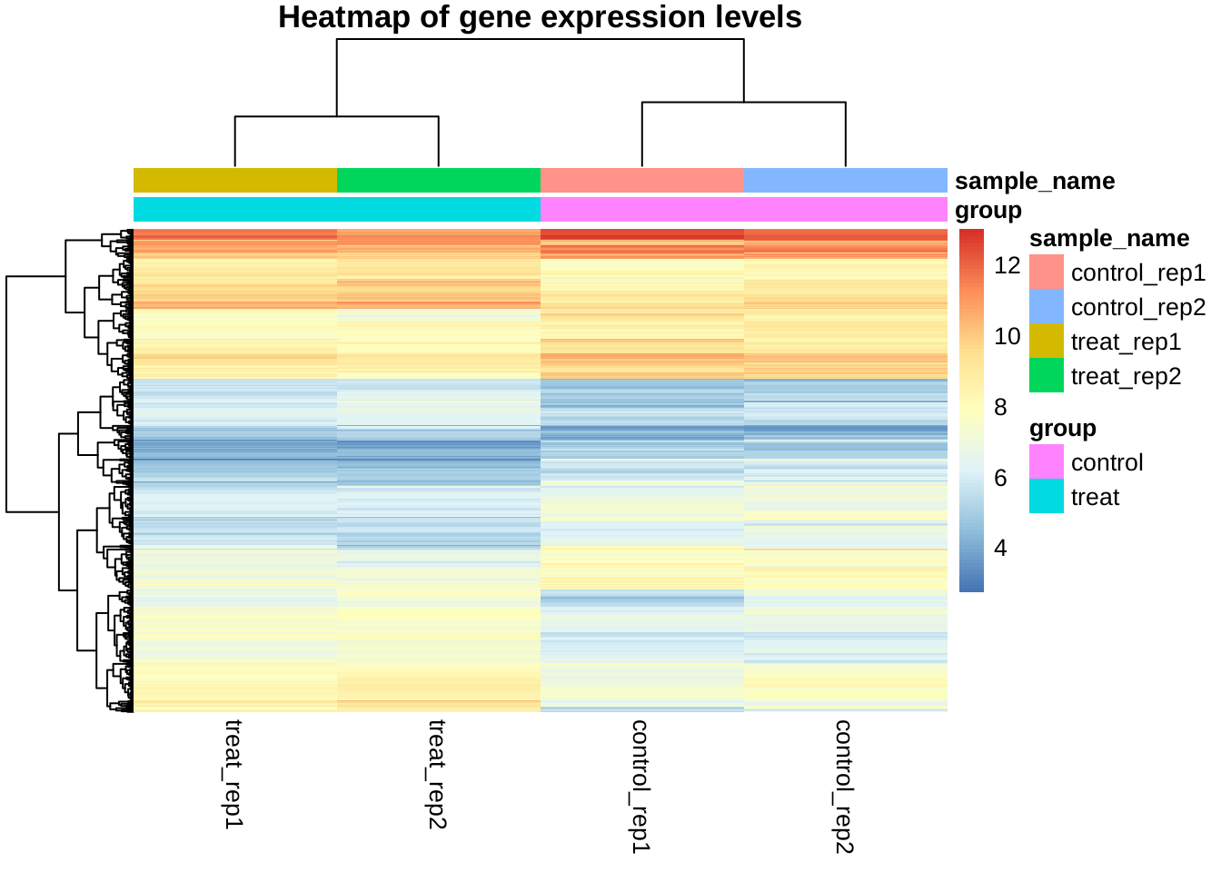
We can roughly divide the genes (probes) into three clusters, and the control/treat samples are also clearly separated.
PCA plot
library(ggfortify)
autoplot(prcomp(exprs(edata)[rownames(selected), ]))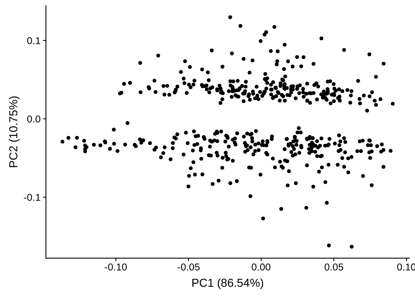
The PCA plot did not provide much useful information.
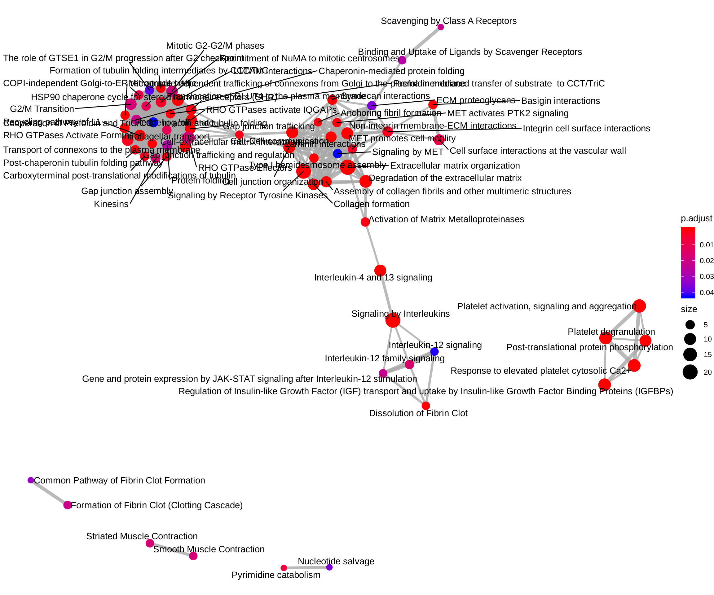
Pathway analysis
library(ReactomePA)## ## ReactomePA v1.24.0 For help: https://guangchuangyu.github.io/ReactomePA
##
## If you use ReactomePA in published research, please cite:
## Guangchuang Yu, Qing-Yu He. ReactomePA: an R/Bioconductor package for reactome pathway analysis and visualization. Molecular BioSystems 2016, 12(2):477-479entrez_ids <- mapIds(hgu95av2.db::hgu95av2.db, keys = rownames(selected),
keytype = "PROBEID", column = "ENTREZID", multiVals = "first")## 'select()' returned 1:many mapping between keys and columnsentrez_ids <- entrez_ids[!is.na(entrez_ids)]
reactome_enrich <- enrichPathway(gene = entrez_ids, organism = "human")barplot(reactome_enrich, showCategory = Inf)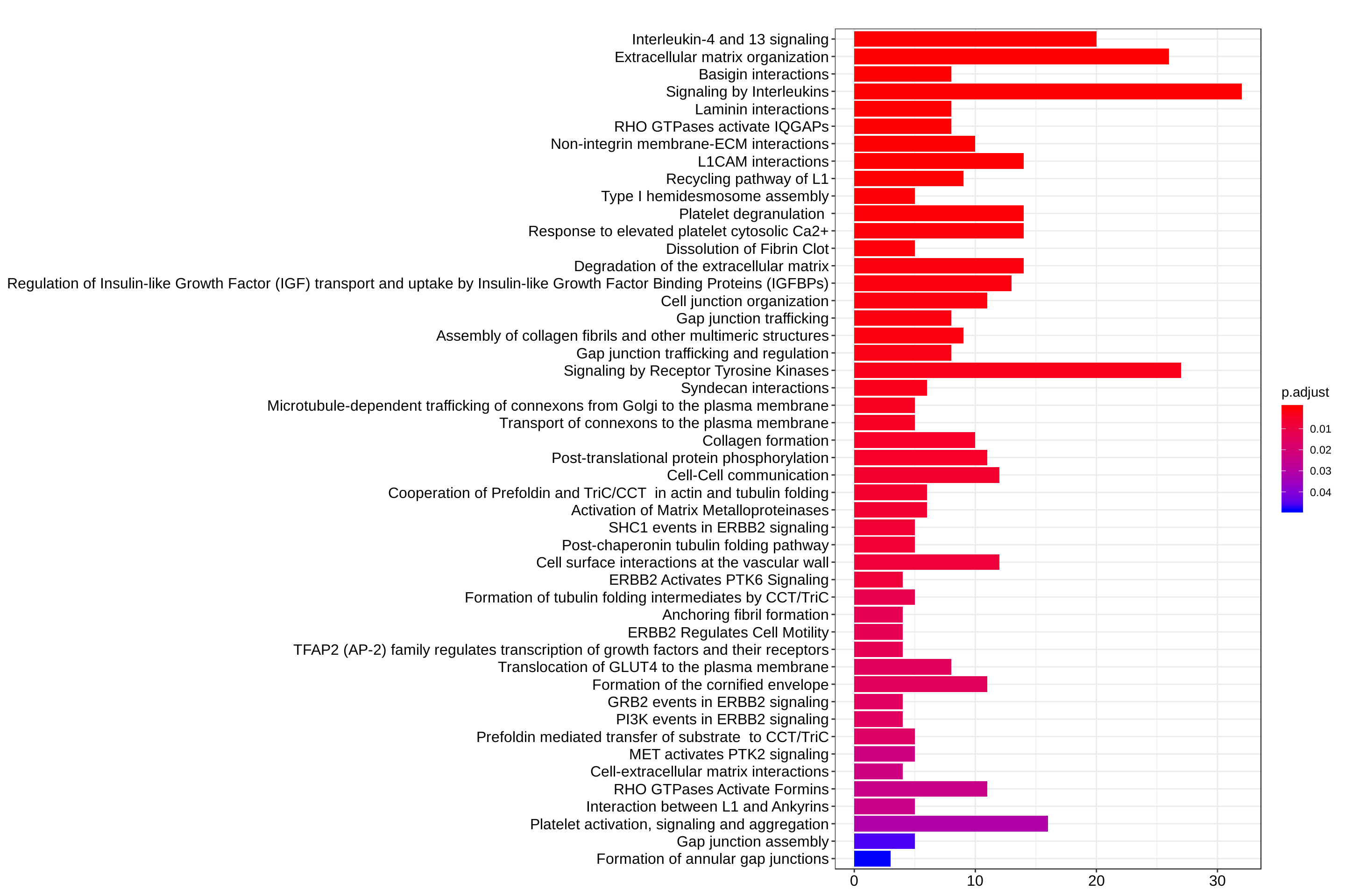
dotplot(reactome_enrich, showCategory = Inf)
ReactomePA::emapplot(reactome_enrich, showCategory = Inf)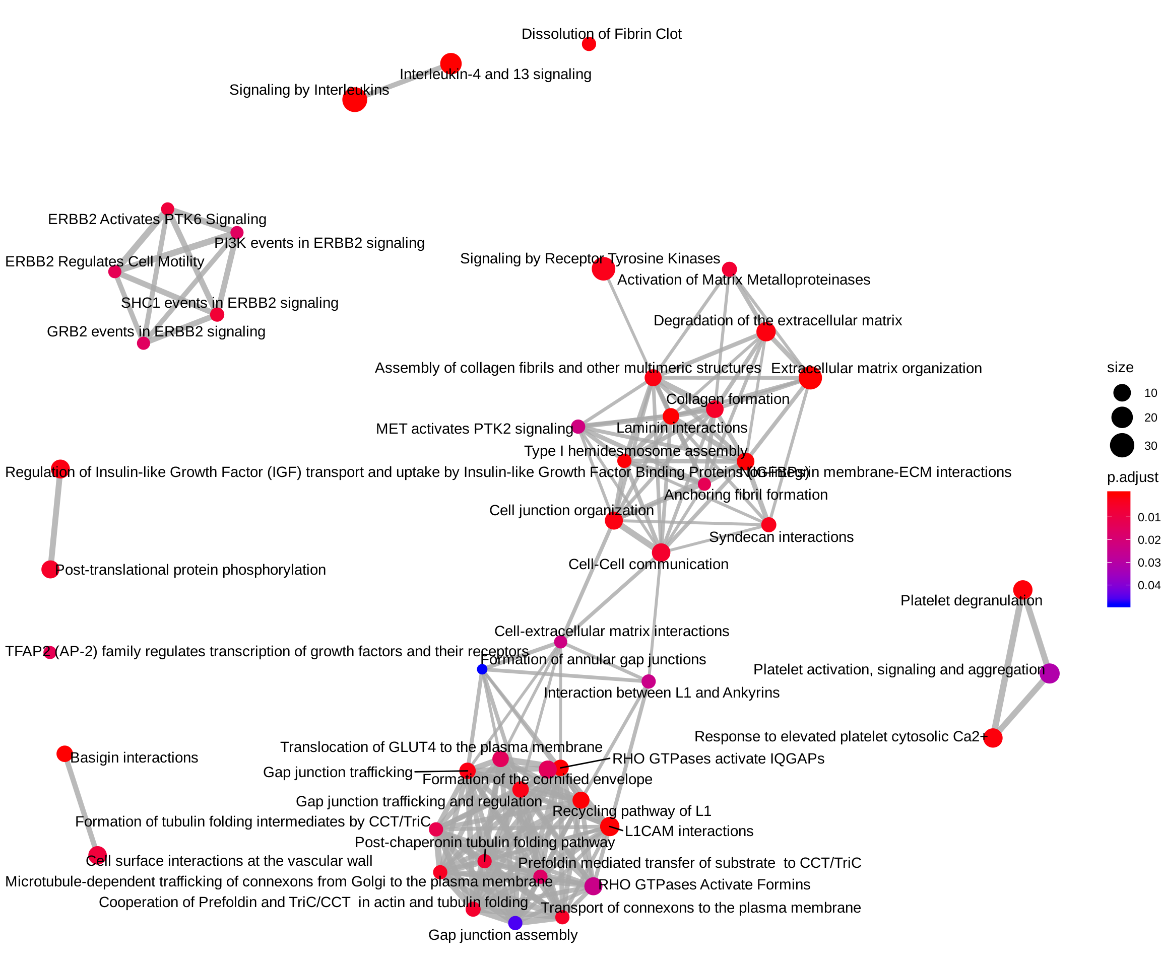
Pathway analysis of up-regulated genes
up_regulated <- selected[selected$logFC > 0, ]
up_regulated <- up_regulated[rownames(up_regulated) %in% names(entrez_ids), ]
ReactomePA::emapplot(
    enrichPathway(gene = entrez_ids[rownames(up_regulated)], organism = "human"),
    showCategory = Inf)
## Using `nicely` as default layout
Pathway analysis of down-regulated genes
down_regulated <- selected[selected$logFC < 0, ]
down_regulated <- down_regulated[rownames(down_regulated) %in% names(entrez_ids), ]
ReactomePA::emapplot(
    enrichPathway(gene = entrez_ids[rownames(down_regulated)], organism = "human"),
    showCategory = Inf)